Introduction.

Urban social movements represent complex networks of relationships between heterogeneous actors who coordinate collective action through multiple types of ties (Diani, 2015). However, not all movement activity carries the same risks and costs for participants. The conflict over Peñalolén’s Master Plan in 2011 provides an exemplary case to analyze how multiplex networks facilitate high-risk activism and enable broad coalition formation among diverse urban actors despite significant personal and organizational costs.

Theoretical Framework

Networks and High-Risk Activism

Our analysis integrates three complementary theoretical perspectives: social movement networks, contentious politics, and high-risk activism. From a network perspective, movements emerge from dense webs of multiplex relationships that facilitate resource mobilization and sustain collective identities (Diani and McAdam 2003; Mische 2003). These networks serve both instrumental and symbolic functions - channeling resources while also cultivating shared interpretive frames (Passy and Giugni 2001).

The contentious politics approach emphasizes how political opportunities and threats trigger episodes of contention through mechanisms like boundary activation and polarization (McAdam, Tarrow, and Tilly 2001; Tilly and Tarrow 2015). These mechanisms operate through relational processes of brokerage and scale shift that connect previously disparate actors into broader coalitions (Tarrow 2005).

However, McAdam (1986) demonstrates that participation in high-risk activism - defined by significant personal costs, potential for repression, and sustained commitment - follows distinct pathways requiring both strong ideological identification and integration into activist networks. In Peñalolén, opposing the Master Plan represented high-risk activism because organizations faced potential repression, required significant resource commitments, and depended on maintaining costly coalitions.

Biographical Availability and Network Integration

Following McAdam (1986), we argue that “biographical availability” - the absence of constraints that increase participation costs - shapes involvement at both individual and organizational levels. This interacts with Gould’s (1991) conception of tie multiplexity as a fundamental mechanism that:

Generates structural resistance to demobilization
Facilitates coordination between diverse actors
Produces mutual reinforcement between different types of relationships

At the micro level, multiple ties between specific organizations reinforce commitments and reduce uncertainty in interactions (Baldassarri & Diani, 2007). At the macro level, multiplexity increases overall network robustness and enables the integration of different organizational clusters while sustaining broader collective identities (Diani 2015).

Boundary Mechanisms and Movement Evolution

Drawing on Tilly (2004), we analyze how boundary change mechanisms shape movement dynamics through:

Inscription-Erasure: The creation/dissolution of social boundaries
Activation-Deactivation: Changes in the salience of existing boundaries
Site Transfer: Relocation of actors relative to boundaries
Relocation: Shifts in boundary-organizing relations

These mechanisms interact with network structures and biographical availability to shape patterns of diffusion and coalition formation (Tilly and Tarrow 2015).

Complex Diffusion and Strong Ties

Recent work on complex contagion demonstrates that the spread of contentious behaviors through networks depends on:

Multiple exposures through redundant ties (Centola and Macy 2007)
Local clustering that provides social reinforcement (Centola 2018)
Strong ties that sustain costly forms of activism (McAdam and Paulsen 1993)

However, McAdam (1986) suggests that strong ties matter more than multiple weak ties for high-risk activism, and that integration into activist networks reduces uncertainty about participation costs.

Hypotheses

Building on this integrated framework, we propose four hypotheses:

H1: Network Structure and Biographical Availability
- Network formation will exhibit significant transitivity (GWESP)
- Organizations with fewer constraints will show higher degree centrality
- Prior activism history will moderate structural position effects
H2: Differentiated Tie Effects
- Strong ties will have greater impact than multiple weak ties
- Trust/values ties will show stronger effects than instrumental ties
- Biographical availability will moderate tie multiplexity effects
H3: Strategic Integration
- Multiple ties increase adoption probability more for constrained organizations
- Integration into activist networks reduces the effect of organizational constraints
- Core-periphery structures emerge from differential biographical availability
H4: Complex Diffusion
- Adoption requires exposure through multiple strong ties
- Local clustering amplifies the effect of strong ties
- Prior activism creates different adoption thresholds
- Temporal dynamics show punctuated rather than gradual adoption

Data and Methods

Research Design

We employ a mixed-methods design (Domínguez and Hollstein 2014) combining social network analysis with qualitative contextual data. Our approach conceptualizes relational structure as a multidimensional space of social positions in which population members are non-randomly distributed (Scott 2011).

Data Collection

Data was collected during 2017-2018 through:

Network Surveys (N=31)
- Name generator limited to 5 nominations
- Multiple tie types
- Organizational attributes
In-depth Interviews (N=12)
- Key informants
- Conflict history
- Coordination dynamics
Documentary Sources
- Local press coverage
- Organizational documents
- Meeting minutes

The sampling strategy combined:

Initial identification of organization types
Snowball sampling until saturation (40% name repetition)
Secondary source validation

Networks and Attributes

We analyze five types of ties between 70 organizations:

Cooperation (joint activities)
Trust (historical bonds)
Resources (material support)
Values (interpretive frames)
Kinship (family ties)

Limitations

Important methodological limitations include:

Temporal bias from retrospective data collection
Potential underrepresentation of peripheral actors
Artificial cap on nominations (5)
Difficulty capturing tie intensity

Estrategia Analítica

Análisis Descriptivo:
- Medidas de centralidad
- Detección de bloques
- Análisis de multiplexidad
Modelación ERGM:
- Efectos estructurales
- Homofilia condicional
- Interacción entre vínculos
Modelo de Difusión:
- Contagio complejo
- Umbrales heterogéneos
- Efectos de estructura local

Resultados

library(tidyverse)
library(igraph)
library(tidygraph)
library(statnet)
library(ergm)
library(ggplot2)
library(network)
library(kableExtra)
library(plotly)
library(gridExtra)
library(viridis)
library(sna)
library(concorR)
library(ggraph)
library(Matrix)
library(patchwork)
library(texreg)

Descriptivos

Red

# Leer y preparar las matrices
coop_matrix <-       as.matrix(read.csv("datos/CoopNet.csv", header=FALSE))
trust_matrix <-      as.matrix(read.csv("datos/ConfianzaNet.csv", header=FALSE))
resources_matrix <-  as.matrix(read.csv("datos/RecursosNet.csv", header=FALSE))
values_matrix <-     as.matrix(read.csv("datos/ValoresNet.csv", header=FALSE))
parentesco_matrix <- as.matrix(read.csv("datos/ParentescoNet.csv", header=FALSE))

# Leer atributos
attributes <- read.csv("datos/Atributos _org2011.csv", header=TRUE)

# Verificar si las redes son dirigidas
is_directed <- list(
  Cooperacion = !isSymmetric(coop_matrix),
  Confianza = !isSymmetric(trust_matrix),
  Recursos = !isSymmetric(resources_matrix),
  Valores = !isSymmetric(values_matrix),
  Parentesco = !isSymmetric(parentesco_matrix)
)

print("Verificación de direccionalidad de las redes:")

[1] "Verificación de direccionalidad de las redes:"

print(unlist(is_directed))

Cooperacion   Confianza    Recursos     Valores  Parentesco 
       TRUE        TRUE        TRUE        TRUE        TRUE

# Lista de todas las matrices para análisis
matrices_list <- list(
  Cooperacion = coop_matrix,
  Confianza = trust_matrix,
  Recursos = resources_matrix,
  Valores = values_matrix,
  Parentesco = parentesco_matrix
)

map_lgl(matrices_list, is.matrix)

Cooperacion   Confianza    Recursos     Valores  Parentesco 
       TRUE        TRUE        TRUE        TRUE        TRUE

map_lgl(matrices_list, function(x) nrow(x) == ncol(x))

Cooperacion   Confianza    Recursos     Valores  Parentesco 
       TRUE        TRUE        TRUE        TRUE        TRUE

print("\nEstadísticas descriptivas de las redes:")

[1] "\nEstadísticas descriptivas de las redes:"

map_dfr(matrices_list, function(x) {
  g <- graph_from_adjacency_matrix(x, mode="directed")
  tibble(
    Densidad = edge_density(g),
    N_lazos = sum(x),
    N_nodos_activos = sum(rowSums(x) > 0),
    Reciprocidad = reciprocity(g),
    Transitivity = transitivity(g),
    Componentes = count_components(g),
    Diametro = diameter(g, directed=TRUE, weights=NA)
  )
}, .id = "Red") %>% 
  kbl() %>%
  kable_paper("hover", full_width = T)

Red	Densidad	N_lazos	N_nodos_activos	Reciprocidad	Transitivity	Componentes	Diametro
Cooperacion	0.0291925	141	32	0.4397163	0.3434705	11	8
Confianza	0.0260870	126	30	0.3492063	0.3807692	15	7
Recursos	0.0198758	96	28	0.2291667	0.2601626	18	7
Valores	0.0271222	131	30	0.4427481	0.3306122	12	8
Parentesco	0.0095238	46	17	0.3043478	0.2553191	41	4

Network Structure and Organizational Field

Our analysis of network structure reveals a clear organizational field configuration characterized by differential density patterns across network types. These patterns suggest a hierarchical integration of the field, where:

Political Organizations Dominance:

MPL (Movimiento de Pobladores en Lucha) shows highest indegree (13)
OCAP (Organización política de base) follows with high centrality (7)
Housing committees (CV_BrillaElSol) maintain significant positions (6)

[Quote opportunity: MPL leader discussing their role in coordinating different organizations]

Actores

# Crear objeto network con atributos
net_coop <- network(coop_matrix, directed=TRUE)

# Agregar atributos a la red
net_coop %v% "tipo" <- attributes$Tipo_de_organización
net_coop %v% "ubicacion" <- attributes$Ubicación
net_coop %v% "orientacion" <- attributes$Orientación

# Calcular medidas de centralidad
cent_df <- data.frame(
  Organizacion = attributes$Nombre,
  Tipo = attributes$Tipo_de_organización,
  Orientacion = attributes$Orientación,
  # Centralidades
  Degree = sna::degree(net_coop, gmode="digraph"),
  Indegree = sna::degree(net_coop, gmode="digraph", cmode="indegree"),
  Outdegree = sna::degree(net_coop, gmode="digraph", cmode="outdegree"),
  Betweenness = sna::betweenness(net_coop),
  Eigenvector = sna::evcent(net_coop)
)

# Top 10 actores más centrales según diferentes medidas
print("Top 10 actores según Indegree:")

[1] "Top 10 actores según Indegree:"

cent_df %>%
  arrange(desc(Indegree)) %>%
  select(Organizacion, Tipo, Indegree) %>%
  head(10) %>%
  kbl() %>%
  kable_paper("hover", full_width = T)

Organizacion	Tipo	Indegree
OPP_MPL	Organización política de pobladores	13
OPB_OCAP	Organización política de base	7
CV_BrillaElSol	Comité de vivienda	6
OC_RAP	Organización cultural	6
OC_Murgarte	Organización cultural	5
OPB_AlexLemún	Organización política de base	5
OPB_RIP	Organización política de base	5
OPB_CristoJoven	Organización política de base	4
OPP_MUA	Organización política de pobladores	4
OV_JJVV_n°19_Bolivar	Organización vecinal	4

print("\nTop 10 actores según Betweenness:")

[1] "\nTop 10 actores según Betweenness:"

cent_df %>%
  arrange(desc(Betweenness)) %>%
  select(Organizacion, Tipo, Betweenness) %>%
  head(10) %>%
  kbl() %>%
  kable_paper("hover", full_width = T)

Organizacion	Tipo	Betweenness
OPP_MPL	Organización política de pobladores	497.7976
OV_JJVV_ComunidadEcológica	Organización vecinal	385.0000
CV_LosColgados	Comité de vivienda	337.7976
OPB_RIP	Organización política de base	218.9643
Gob_Mun	Otros	199.0000
OPB_AlexLemún	Organización política de base	198.4405
CV_BrillaElSol	Comité de vivienda	176.3214
OPB_OCAP	Organización política de base	134.9405
OPP_MUA	Organización política de pobladores	125.4881
OPB_CristoJoven	Organización política de base	113.5714

# Análisis de centralidad por tipo de organización
cent_by_type <- cent_df %>%
  group_by(Tipo) %>%
  summarise(
    Mean_Indegree = mean(Indegree),
    Mean_Betweenness = mean(Betweenness),
    N = n()
  )

print("\nCentralidad promedio por tipo de organización:")

[1] "\nCentralidad promedio por tipo de organización:"

cent_by_type %>%
  kbl() %>%
  kable_paper("hover", full_width = T)

Tipo	Mean_Indegree	Mean_Betweenness	N
Club deportivo	0.750000	0.00000	4
Comité de vivienda	2.444444	60.16138	9
Organización cultural	1.923077	24.18498	13
Organización política de base	4.166667	119.85119	6
Organización política de pobladores	4.333333	126.24008	6
Organización vecinal	1.111111	22.11464	27
Otros	2.000000	51.90000	5

Structural Differentiation: Core political organizations average higher betweenness centrality (119.85 for political base organizations, 126.24 for pobladores organizations) compared to neighborhood organizations (22.11).

Equivalencia estructural

The CONCOR analysis identified four distinct blocks:

Political-Strategic Block (18 organizations):

9 Housing Committees
4 Cultural Organizations
4 Sports Clubs
1 Municipal Actor

Cultural-Tactical Block (13 organizations):

8 Cultural Organizations
1 Political Base Organization
4 Others

Base Organization Block (14 organizations):

6 Pobladores Organizations
5 Base Political Organizations
3 Neighborhood Organizations

Neighborhood Block (15 organizations):

Exclusively neighborhood organizations

[Quote opportunity: Description of different organizational roles in the movement]

# Leer datos
coop_matrix <- as.matrix(read.csv("datos/CoopNet.csv", header=FALSE))
attributes <- read.csv("datos/Atributos _org2011.csv", header=TRUE)

# Realizar CONCOR
bloques <- concor(list(coop_matrix), cutoff=0.8, nsplit=2)

# Ver composición de los bloques
for(i in 1:4) {
    cat(paste("\n\nBLOQUE", i, "\n"))
    cat("---------------\n")
    organizaciones <- attributes[bloques == i, ]
    print(table(organizaciones$Tipo))
    cat("\nOrganizaciones específicas:\n")
    print(organizaciones$Nombre)
}



BLOQUE 1 
---------------

2 5 6 7 
9 4 4 1 

Organizaciones específicas:
 [1] "CD_AvanceDeCarvallo"       "CD_CristoJovén"           
 [3] "CD_RealHéroes"             "CD_SanLuisDelElqui"       
 [5] "CV_BrillaElSol"            "CV_CaminoALaVictoria"     
 [7] "CV_CasaDigna"              "CV_CoordAllegados"        
 [9] "CV_LosColgados"            "CV_PasoSeguro"            
[11] "CV_PorUnaVidaMejor"        "CV_UnaEsperanzaEnElFuturo"
[13] "CV_volverAEmpezar"         "Gob_Mun"                  
[15] "OC_ ClubCientífico"        "OC_Barracón"              
[17] "OC_CircoChino"             "OC_EncuentroAndino"       


BLOQUE 2 
---------------

4 5 7 
1 8 4 

Organizaciones específicas:
 [1] "OC_GenteDelSur"            "OC_ManzoPiño"             
 [3] "OC_Murgarte"               "OC_PasiónPorMiTierra"     
 [5] "OC_PorLaMemoriaHistórica"  "OC_RadioEncuentro(tv8)"   
 [7] "OC_RAP"                    "OC_Yanawara"              
 [9] "OG_ColegioDeArquitectos"   "ONG_DefendamosLaCiudad"   
[11] "ONG_PACc"                  "OP_AsociaciónMicrobuseros"
[13] "OPB_AlexLemún"            


BLOQUE 3 
---------------

1 3 4 
3 6 5 

Organizaciones específicas:
 [1] "OPB_CristoJoven"             "OPB_GrfemAuto"              
 [3] "OPB_OCAP"                    "OPB_RecupHermida"           
 [5] "OPB_RIP"                     "OPP_FENAPO"                 
 [7] "OPP_MPL"                     "OPP_MPLD"                   
 [9] "OPP_MPST"                    "OPP_MUA"                    
[11] "OPP_PIgualdad"               "OV_AP_LosJardinesDeVespucio"
[13] "OV_CD_ReactivaciónEnMasas"   "OV_CD_VillaSolNaciente"     


BLOQUE 4 
---------------

 1 
15 

Organizaciones específicas:
 [1] "OV_ComSeguridadSM"               "OV_CVD_VillaAlboradaNuevaPalena"
 [3] "OV_JI_ManosyNaturaleza"          "OV_JJVV_ComunidadEcológica"     
 [5] "OV_JJVV_CordilleraNevada"        "OV_JJVV_LaCordillera"           
 [7] "OV_JJVV_n°11_LaFaena"            "OV_JJVV_n°12_LaFaena"           
 [9] "OV_JJVV_n°14_Parque1"            "OV_JJVV_n°17_IsabelRiquelme"    
[11] "OV_JJVV_n°18"                    "OV_JJVV_n°19_Bolivar"           
[13] "OV_JJVV_n°19_Heroes"             "OV_JJVV_n°29_LoHerAlto"         
[15] "OV_JJVV_PortalDelSol"

# Calcular densidades entre bloques
block_density <- matrix(0, 4, 4)
for(i in 1:4) {
    for(j in 1:4) {
        nodes_i <- which(bloques == i)
        nodes_j <- which(bloques == j)
        if(length(nodes_i) > 0 && length(nodes_j) > 0) {
            block_density[i,j] <- sum(coop_matrix[nodes_i, nodes_j]) / 
                                 (length(nodes_i) * length(nodes_j))
        }
    }
}

# Mostrar densidades
cat("\n\nDensidad entre bloques:\n")



Densidad entre bloques:

print(round(block_density, 3))

      [,1]  [,2]  [,3]  [,4]
[1,] 0.056 0.009 0.044 0.022
[2,] 0.000 0.077 0.033 0.026
[3,] 0.048 0.044 0.112 0.010
[4,] 0.007 0.026 0.024 0.036

# Calcular cohesión de bloques
for(i in 1:4) {
    cat(paste("\n\nCohesión Bloque", i, "\n"))
    internal <- block_density[i,i]
    external <- mean(block_density[i,-i])
    ei_index <- (external - internal)/(external + internal)
    cat(paste("Densidad interna:", round(internal, 3), "\n"))
    cat(paste("Densidad externa media:", round(external, 3), "\n"))
    cat(paste("Índice E-I:", round(ei_index, 3), "\n"))
}



Cohesión Bloque 1 
Densidad interna: 0.056 
Densidad externa media: 0.025 
Índice E-I: -0.383 


Cohesión Bloque 2 
Densidad interna: 0.077 
Densidad externa media: 0.02 
Índice E-I: -0.595 


Cohesión Bloque 3 
Densidad interna: 0.112 
Densidad externa media: 0.034 
Índice E-I: -0.538 


Cohesión Bloque 4 
Densidad interna: 0.036 
Densidad externa media: 0.019 
Índice E-I: -0.305

# 1. Preparar datos para el heatmap de densidades entre bloques
density_df <- expand.grid(
  from = factor(1:4, labels = paste("Bloque", 1:4)),
  to = factor(1:4, labels = paste("Bloque", 1:4))
) %>%
  mutate(density = as.vector(block_density))



# 2. Preparar datos para la composición de bloques
composicion_bloques <- data.frame(
  Bloque = rep(1:4, c(18, 13, 14, 15)),
  Tipo = c(
    rep(c("Comite Vivienda","Org. Cultural","Club Deportivo","Gob. Municipal"), c(9,4,4,1)), # Bloque 1
    rep(c("Org. Política Base","Org. Cultural","Otros"), c(1,8,4)), # Bloque 2
    rep(c("Org. Vecinal","Org. Política Pobladores","Org. Política Base"), c(3,6,5)), # Bloque 3
    rep("Org. vecinal", 15) # Bloque 4
  )
)

# 3. Preparar datos para métricas de cohesión
cohesion_df <- data.frame(
  Bloque = factor(1:4, labels = paste("Bloque", 1:4)),
  Densidad_interna = diag(block_density),
  Densidad_externa = sapply(1:4, function(i) mean(block_density[i,-i])),
  EI_index = sapply(1:4, function(i) {
    internal <- block_density[i,i]
    external <- mean(block_density[i,-i])
    (external - internal)/(external + internal)
  })
) %>%
  pivot_longer(cols = -Bloque, 
               names_to = "Metrica", 
               values_to = "Valor")

# Crear las visualizaciones

# 1. Heatmap de densidades
p1 <- ggplot(density_df, aes(x = from, y = to, fill = density)) +
  geom_tile() +
  scale_fill_viridis() +
  labs(title = "Densidad entre Bloques",
       x = "Bloque Origen",
       y = "Bloque Destino",
       fill = "Densidad") +
  theme_minimal() +
  theme(axis.text.x = element_text(angle = 45, hjust = 1))

# 2. Composición de bloques
p2 <- ggplot(composicion_bloques, aes(x = factor(Bloque), fill = Tipo)) +
  geom_bar(position = "fill") +
  scale_fill_viridis_d() +
  labs(title = "Composición de Bloques",
       x = "Bloque",
       y = "Proporción",
       fill = "Tipo de Organización") +
  theme_minimal()

# 3. Métricas de cohesión
p3 <- ggplot(cohesion_df, aes(x = Bloque, y = Valor, fill = Metrica)) +
  geom_bar(stat = "identity", position = "dodge") +
  scale_fill_viridis_d() +
  labs(title = "Métricas de Cohesión por Bloque",
       x = "Bloque",
       y = "Valor",
       fill = "Métrica") +
  theme_minimal()

# Convertir a plotly
p1_plotly <- ggplotly(p1)
p2_plotly <- ggplotly(p2)
p3_plotly <- ggplotly(p3)

# Mostrar los plots
p1_plotly

p2_plotly

p3_plotly

# Create multiplex network
multiplex_matrix <- coop_matrix * 0.3 + 
                   trust_matrix * 0.3 + 
                   resources_matrix * 0.2 + 
                   values_matrix * 0.2

# Create graph
g <- graph_from_adjacency_matrix(multiplex_matrix, mode="directed", weighted=TRUE)

# Add vertex attributes using existing data
V(g)$degree <- igraph::degree(g)
V(g)$betweenness <- igraph::betweenness(g)
V(g)$eigenvector <- eigen_centrality(g)$vector
V(g)$block <- attributes$X1PosciónCONCOR
V(g)$type <- attributes$Tipo_de_organización
V(g)$orientation <- attributes$Orientación
V(g)$nombre <- attributes$Nombre


# Add edge attributes
edge_list <- as_edgelist(g)
E(g)$block_tie <- ifelse(
  V(g)$block[edge_list[,1]] == V(g)$block[edge_list[,2]], 
  paste0("Block", V(g)$block[edge_list[,1]]), 
  "between"
)

# Network plot with ggraph
p1 <- ggraph(g, layout = "fr") +
  geom_edge_link(aes(alpha = ifelse(V(g)$block[from] == V(g)$block[to], 0.6, 0.2)),
                 color = "black",
                 arrow = arrow(length = unit(2, 'mm'))) +
  geom_node_point(aes(size = betweenness,
                     color = as.factor(block)),
                 alpha = 0.7) +
  geom_node_label(aes(label = ifelse(betweenness > quantile(betweenness, 0.92),
                                    nombre, "")),
                 repel = TRUE,
                 size = 3) +
  scale_color_viridis_d(option = "D",
                       name = "Bloque",
                       labels = c("Político", "JJ.VV", "Base", "Cultural")) +
  scale_size_continuous(name = "Intermediación",
                       range = c(2, 8),
                       breaks = c(0, 0.025, 0.05, 0.075, 0.1, 0.125),
                       labels = c("0.000", "0.025", "0.050", "0.075", "0.100", "0.125")) +
  guides(color = guide_legend(override.aes = list(size = 5)),
         size = guide_legend(override.aes = list(alpha = 1)),
         edge_alpha = guide_legend(title = "Vinculo")) +  # Eliminamos el título de la leyenda edge_alpha
  labs(title = "") +
  theme_graph() +
  theme(legend.position = "right",
        plot.title = element_text(hjust = 0.5, size = 14),
        legend.text = element_text(size = 10),
        legend.title = element_text(size = 12)) 

print(p1)

This suggests:

Integration occurs through nested hierarchies
Cultural organizations serve as brokers
Political organizations maintain core-periphery structure

This extends Diani’s (2015) movement integration theory by specifying:

The role of organizational heterogeneity
The importance of cultural brokers
The hierarchical nature of integration

ERGM

# Verificar distribución de grados
out_degrees <- sna::degree(net_coop)
table(out_degrees)

out_degrees
 0  1  2  3  4  5  6  7  8  9 10 11 12 14 19 
10 20  7  6  2  1  5  4  1  7  1  3  1  1  1

max(out_degrees)

[1] 19

# Agregar constraints para manejar el límite de nominaciones
model2 <- ergm(net_coop ~ 
               edges + 
               gwesp(0.25, fixed = TRUE) + 
               gwidegree(0.25, fixed=TRUE) + 
               #gwdegree(0.25, fixed = TRUE) +
               edgecov(trust_matrix) + 
               edgecov(resources_matrix) +
               edgecov(parentesco_matrix) +
               #nodefactor("tipo") +
               #nodefactor("orientacion") +
               #nodefactor("ubicacion") +
               nodematch("tipo") + 
               nodematch("orientacion", diff=TRUE) +
               nodematch("ubicacion"),
               constraints = ~bd(maxout=max(out_degrees)), 
               control = control.ergm(seed = 123,
                                    MCMLE.maxit = 25, # Aumentar iteraciones 
                                    MCMC.burnin = 5000, # Aumentar burn-in
                                    MCMC.interval = 100, # Aumentar intervalo
                                    MCMC.samplesize = 10000, # Aumentar tamaño de muestra
                                    parallel = 8,
                                    parallel.type = "PSOCK"))
summary(model2)

Call:
ergm(formula = net_coop ~ edges + gwesp(0.25, fixed = TRUE) + 
    gwidegree(0.25, fixed = TRUE) + edgecov(trust_matrix) + edgecov(resources_matrix) + 
    edgecov(parentesco_matrix) + nodematch("tipo") + nodematch("orientacion", 
    diff = TRUE) + nodematch("ubicacion"), constraints = ~bd(maxout = max(out_degrees)), 
    control = control.ergm(seed = 123, MCMLE.maxit = 25, MCMC.burnin = 5000, 
        MCMC.interval = 100, MCMC.samplesize = 10000, parallel = 8, 
        parallel.type = "PSOCK"))

Monte Carlo Maximum Likelihood Results:

                                     Estimate Std. Error MCMC % z value
edges                                -7.38970    0.56304      0 -13.125
gwesp.OTP.fixed.0.25                  1.89059    0.27185      0   6.955
gwideg.fixed.0.25                     2.23302    0.69071      0   3.233
edgecov.trust_matrix                  6.37713    0.79292      0   8.043
edgecov.resources_matrix              5.53576    1.04376      0   5.304
edgecov.parentesco_matrix            -2.94786    0.94623      0  -3.115
nodematch.tipo                        0.37669    0.41694      0   0.903
nodematch.orientacion.Conflictiva     0.32523    0.48308      0   0.673
nodematch.orientacion.No_conflictiva  0.03196    0.51924      0   0.062
nodematch.ubicacion                   0.40242    0.41824      0   0.962
                                     Pr(>|z|)    
edges                                 < 1e-04 ***
gwesp.OTP.fixed.0.25                  < 1e-04 ***
gwideg.fixed.0.25                     0.00123 ** 
edgecov.trust_matrix                  < 1e-04 ***
edgecov.resources_matrix              < 1e-04 ***
edgecov.parentesco_matrix             0.00184 ** 
nodematch.tipo                        0.36628    
nodematch.orientacion.Conflictiva     0.50079    
nodematch.orientacion.No_conflictiva  0.95092    
nodematch.ubicacion                   0.33596    
---
Signif. codes:  0 '***' 0.001 '**' 0.01 '*' 0.05 '.' 0.1 ' ' 1

     Null Deviance:     0  on 4830  degrees of freedom
 Residual Deviance: -5231  on 4820  degrees of freedom
 
Note that the null model likelihood and deviance are defined to be 0.
This means that all likelihood-based inference (LRT, Analysis of
Deviance, AIC, BIC, etc.) is only valid between models with the same
reference distribution and constraints.

AIC: -5211  BIC: -5147  (Smaller is better. MC Std. Err. = 12.24)

# Print summary
htmlreg(model2,
        stars=c(0.01,0.05,0.1), 
        digits=3, 
        star.symbol='&#42;',
        custom.note = paste("%stars."),
         align.center=TRUE,
        single.row = T, 
        bold = 0.05)

Warning in nobs.ergm(object): The number of observed dyads in this network is
ill-defined due to complex constraints on the sample space. Disable this
warning with 'options(ergm.loglik.warn_dyads=FALSE)'.

Statistical models
	Model 1
edges	-7.390 (0.563)^***
gwesp.OTP.fixed.0.25	1.891 (0.272)^***
gwideg.fixed.0.25	2.233 (0.691)^***
edgecov.trust_matrix	6.377 (0.793)^***
edgecov.resources_matrix	5.536 (1.044)^***
edgecov.parentesco_matrix	-2.948 (0.946)^***
nodematch.tipo	0.377 (0.417)
nodematch.orientacion.Conflictiva	0.325 (0.483)
nodematch.orientacion.No_conflictiva	0.032 (0.519)
nodematch.ubicacion	0.402 (0.418)
AIC	-5211.484
BIC	-5146.658
Log Likelihood	2615.742
^*p < 0.01; ^p < 0.05; ^*p < 0.1.

Trust-Based Diffusion: The strongest positive effect (6.423***) comes from trust networks, supporting Passy & Monsch’s (2014) argument that identity transformation occurs primarily through trust relationships. Your case shows how historical relationships between pobladores organizations provided the foundation for contentious identity spread.

[Quote opportunity: Leader discussing how long-term trust relationships facilitated political alignment]

Resource Network Amplification: The strong positive effect of resource ties (5.513) indicates that material interdependencies reinforced identity diffusion, consistent with Diani’s (2015) findings about movement infrastructure. In Peñalolén, resource sharing created durable channels for identity transmission.

Kinship Network Constraint: The negative effect of kinship ties (-3.082) suggests these relationships actually inhibited contention diffusion, contrasting with some social movement literature but aligning with Gould’s (1991) findings about the primacy of political over personal ties in contentious episodes.

Triadic Closure: Significant GWESP effect (1.899) indicates importance of local clustering in network formation. The significant GWESP effect combined with trust-resource complementarity suggests a new theoretical mechanism: “networked capacity building”, where:

Local clustering provides social validation
Multiple ties build organizational capacity
Different tie types serve distinct but complementary functions

# Assess goodness-of-fit  
gof <- gof(model2)
print(gof)


Goodness-of-fit for in-degree 

          obs min  mean max MC p-value
idegree0   12   7 11.49  16       1.00
idegree1   24  19 25.95  33       0.58
idegree2   15   8 14.88  21       1.00
idegree3    8   2  5.99  10       0.40
idegree4    4   2  5.28   8       0.52
idegree5    3   0  2.07   5       0.68
idegree6    2   0  1.72   4       1.00
idegree7    1   0  1.26   3       1.00
idegree8    0   0  0.34   2       1.00
idegree9    0   0  0.02   1       1.00
idegree13   1   0  0.17   1       0.34
idegree14   0   0  0.61   1       0.78
idegree15   0   0  0.18   1       1.00
idegree16   0   0  0.04   1       1.00

Goodness-of-fit for out-degree 

          obs min  mean max MC p-value
odegree0   38  29 33.51  39       0.06
odegree1    3   1  6.00  10       0.16
odegree2    1   0  2.52   6       0.44
odegree3    6   1  4.40   8       0.52
odegree4    4   4  8.30  13       0.08
odegree5    9   6  9.48  16       1.00
odegree6    6   1  4.41   9       0.44
odegree7    3   0  1.10   5       0.16
odegree8    0   0  0.25   2       1.00
odegree9    0   0  0.02   1       1.00
odegree10   0   0  0.01   1       1.00

Goodness-of-fit for edgewise shared partner 

         obs min  mean max MC p-value
esp.OTP0  51  42 51.66  61       0.94
esp.OTP1  53  38 51.78  65       0.88
esp.OTP2  23  17 27.63  39       0.34
esp.OTP3  10   2  7.16  16       0.32
esp.OTP4   4   0  2.78   6       0.52
esp.OTP5   0   0  0.26   2       1.00
esp.OTP6   0   0  0.01   1       1.00

Goodness-of-fit for minimum geodesic distance 

     obs  min    mean  max MC p-value
1    141  130  141.28  152       0.94
2    250  186  243.93  320       0.74
3    283  200  297.23  450       0.84
4    230  149  261.67  358       0.52
5    153   53  172.37  270       0.86
6    117    5   90.04  238       0.60
7     67    0   47.48  175       0.68
8     12    0   26.30  123       0.98
9      0    0   14.57  105       0.96
10     0    0    6.69   75       1.00
11     0    0    2.87   60       1.00
12     0    0    1.64   37       1.00
13     0    0    0.40   13       1.00
14     0    0    0.06    4       1.00
Inf 3577 2972 3523.47 3991       0.94

Goodness-of-fit for model statistics 

                                           obs       min      mean       max
edges                                141.00000 130.00000 141.28000 152.00000
gwesp.OTP.fixed.0.25                  98.91267  80.00013  98.52341 121.90688
gwideg.fixed.0.25                     66.58862  62.14383  66.72183  71.08712
edgecov.trust_matrix                 118.00000 111.00000 118.23000 122.00000
edgecov.resources_matrix              93.00000  91.00000  93.00000  95.00000
edgecov.parentesco_matrix             38.00000  33.00000  38.26000  41.00000
nodematch.tipo                        58.00000  48.00000  58.17000  65.00000
nodematch.orientacion.Conflictiva     65.00000  58.00000  65.26000  77.00000
nodematch.orientacion.No_conflictiva  32.00000  27.00000  32.21000  39.00000
nodematch.ubicacion                   80.00000  72.00000  80.31000  88.00000
                                     MC p-value
edges                                      0.94
gwesp.OTP.fixed.0.25                       0.88
gwideg.fixed.0.25                          0.98
edgecov.trust_matrix                       1.00
edgecov.resources_matrix                   1.00
edgecov.parentesco_matrix                  1.00
nodematch.tipo                             1.00
nodematch.orientacion.Conflictiva          1.00
nodematch.orientacion.No_conflictiva       1.00
nodematch.ubicacion                        1.00

plot(gof)

# Plot diagnostics  
mcmc.diagnostics(model2)

Sample statistics summary:

Iterations = 71040:947712
Thinning interval = 288 
Number of chains = 8 
Sample size per chain = 3045 

1. Empirical mean and standard deviation for each variable,
   plus standard error of the mean:

                                         Mean    SD Naive SE Time-series SE
edges                                 0.05903 5.075 0.032517        0.12296
gwesp.OTP.fixed.0.25                 -0.10569 7.346 0.047069        0.19970
gwideg.fixed.0.25                     0.02225 2.320 0.014863        0.03148
edgecov.trust_matrix                 -0.07521 2.212 0.014171        0.09417
edgecov.resources_matrix              0.14130 1.040 0.006661        0.03974
edgecov.parentesco_matrix            -0.02849 1.760 0.011275        0.06928
nodematch.tipo                       -0.39228 3.238 0.020745        0.09836
nodematch.orientacion.Conflictiva    -0.08140 3.115 0.019958        0.08647
nodematch.orientacion.No_conflictiva  0.03222 2.480 0.015893        0.04188
nodematch.ubicacion                  -0.03645 3.423 0.021934        0.07664

2. Quantiles for each variable:

                                        2.5%    25%       50%   75%  97.5%
edges                                -10.000 -3.000  0.000000 3.000 10.000
gwesp.OTP.fixed.0.25                 -14.072 -5.183 -0.226103 4.770 14.703
gwideg.fixed.0.25                     -4.421 -1.553  0.002064 1.576  4.643
edgecov.trust_matrix                  -4.000 -2.000  0.000000 1.000  4.000
edgecov.resources_matrix              -2.000  0.000  0.000000 1.000  2.000
edgecov.parentesco_matrix             -4.000 -1.000  0.000000 1.000  3.000
nodematch.tipo                        -7.000 -3.000  0.000000 2.000  6.000
nodematch.orientacion.Conflictiva     -6.000 -2.000  0.000000 2.000  6.000
nodematch.orientacion.No_conflictiva  -4.000 -2.000  0.000000 2.000  5.000
nodematch.ubicacion                   -7.000 -2.000  0.000000 2.000  7.000


Are sample statistics significantly different from observed?
               edges gwesp.OTP.fixed.0.25 gwideg.fixed.0.25
diff.      0.0590312           -0.1056921        0.02224916
test stat. 0.4953463           -0.5388267        0.72324454
P-val.     0.6203557            0.5900064        0.46952966
           edgecov.trust_matrix edgecov.resources_matrix
diff.               -0.07520525             0.1412972085
test stat.          -0.80357326             3.5728375854
P-val.               0.42164347             0.0003531338
           edgecov.parentesco_matrix nodematch.tipo
diff.                    -0.02848933  -3.922824e-01
test stat.               -0.41662796  -4.152104e+00
P-val.                    0.67695056   3.294327e-05
           nodematch.orientacion.Conflictiva
diff.                            -0.08140394
test stat.                       -0.94403122
P-val.                            0.34515370
           nodematch.orientacion.No_conflictiva nodematch.ubicacion
diff.                                0.03222496          -0.0364532
test stat.                           0.83536458          -0.4977463
P-val.                               0.40351247           0.6186629
                 (Omni)
diff.                NA
test stat. 9.269142e+01
P-val.     4.232061e-15

Sample statistics cross-correlations:
                                         edges gwesp.OTP.fixed.0.25
edges                                1.0000000            0.7530050
gwesp.OTP.fixed.0.25                 0.7530050            1.0000000
gwideg.fixed.0.25                    0.6327218            0.1914243
edgecov.trust_matrix                 0.4741885            0.4445378
edgecov.resources_matrix             0.2780134            0.1642299
edgecov.parentesco_matrix            0.3676731            0.3838466
nodematch.tipo                       0.6162774            0.5313572
nodematch.orientacion.Conflictiva    0.6096972            0.6467012
nodematch.orientacion.No_conflictiva 0.4621659            0.1876291
nodematch.ubicacion                  0.6745765            0.5925304
                                     gwideg.fixed.0.25 edgecov.trust_matrix
edges                                        0.6327218            0.4741885
gwesp.OTP.fixed.0.25                         0.1914243            0.4445378
gwideg.fixed.0.25                            1.0000000            0.2030942
edgecov.trust_matrix                         0.2030942            1.0000000
edgecov.resources_matrix                     0.1097059            0.1949832
edgecov.parentesco_matrix                    0.1532654            0.7837850
nodematch.tipo                               0.3464443            0.4800150
nodematch.orientacion.Conflictiva            0.1959696            0.4324565
nodematch.orientacion.No_conflictiva         0.4557658            0.1250061
nodematch.ubicacion                          0.3858819            0.2742058
                                     edgecov.resources_matrix
edges                                              0.27801343
gwesp.OTP.fixed.0.25                               0.16422990
gwideg.fixed.0.25                                  0.10970585
edgecov.trust_matrix                               0.19498324
edgecov.resources_matrix                           1.00000000
edgecov.parentesco_matrix                          0.23852542
nodematch.tipo                                     0.16871155
nodematch.orientacion.Conflictiva                  0.20906270
nodematch.orientacion.No_conflictiva               0.03957557
nodematch.ubicacion                                0.23585971
                                     edgecov.parentesco_matrix nodematch.tipo
edges                                              0.367673129      0.6162774
gwesp.OTP.fixed.0.25                               0.383846586      0.5313572
gwideg.fixed.0.25                                  0.153265412      0.3464443
edgecov.trust_matrix                               0.783784955      0.4800150
edgecov.resources_matrix                           0.238525422      0.1687115
edgecov.parentesco_matrix                          1.000000000      0.3806598
nodematch.tipo                                     0.380659797      1.0000000
nodematch.orientacion.Conflictiva                  0.364194350      0.4356268
nodematch.orientacion.No_conflictiva              -0.002733412      0.3402146
nodematch.ubicacion                                0.224005765      0.4544490
                                     nodematch.orientacion.Conflictiva
edges                                                      0.609697174
gwesp.OTP.fixed.0.25                                       0.646701168
gwideg.fixed.0.25                                          0.195969603
edgecov.trust_matrix                                       0.432456453
edgecov.resources_matrix                                   0.209062701
edgecov.parentesco_matrix                                  0.364194350
nodematch.tipo                                             0.435626773
nodematch.orientacion.Conflictiva                          1.000000000
nodematch.orientacion.No_conflictiva                      -0.000845317
nodematch.ubicacion                                        0.321886937
                                     nodematch.orientacion.No_conflictiva
edges                                                         0.462165871
gwesp.OTP.fixed.0.25                                          0.187629091
gwideg.fixed.0.25                                             0.455765800
edgecov.trust_matrix                                          0.125006101
edgecov.resources_matrix                                      0.039575571
edgecov.parentesco_matrix                                    -0.002733412
nodematch.tipo                                                0.340214645
nodematch.orientacion.Conflictiva                            -0.000845317
nodematch.orientacion.No_conflictiva                          1.000000000
nodematch.ubicacion                                           0.305044228
                                     nodematch.ubicacion
edges                                          0.6745765
gwesp.OTP.fixed.0.25                           0.5925304
gwideg.fixed.0.25                              0.3858819
edgecov.trust_matrix                           0.2742058
edgecov.resources_matrix                       0.2358597
edgecov.parentesco_matrix                      0.2240058
nodematch.tipo                                 0.4544490
nodematch.orientacion.Conflictiva              0.3218869
nodematch.orientacion.No_conflictiva           0.3050442
nodematch.ubicacion                            1.0000000

Sample statistics auto-correlation:
Chain 1 
             edges gwesp.OTP.fixed.0.25 gwideg.fixed.0.25 edgecov.trust_matrix
Lag 0    1.0000000            1.0000000         1.0000000            1.0000000
Lag 288  0.6105278            0.7662404         0.3578027            0.9592593
Lag 576  0.4476652            0.6257042         0.1838858            0.9208339
Lag 864  0.3916935            0.5345760         0.1490930            0.8839554
Lag 1152 0.3529669            0.4653355         0.1419611            0.8507835
Lag 1440 0.3290860            0.4256702         0.1182926            0.8191031
         edgecov.resources_matrix edgecov.parentesco_matrix nodematch.tipo
Lag 0                   1.0000000                 1.0000000      1.0000000
Lag 288                 0.9401563                 0.9442878      0.6942477
Lag 576                 0.8863492                 0.8950052      0.5739219
Lag 864                 0.8437976                 0.8527794      0.5279364
Lag 1152                0.8031677                 0.8118708      0.4703870
Lag 1440                0.7658321                 0.7755099      0.4382134
         nodematch.orientacion.Conflictiva nodematch.orientacion.No_conflictiva
Lag 0                            1.0000000                            1.0000000
Lag 288                          0.7424270                            0.5013595
Lag 576                          0.6121624                            0.3280111
Lag 864                          0.5369358                            0.2795610
Lag 1152                         0.4845486                            0.2520274
Lag 1440                         0.4466610                            0.2137526
         nodematch.ubicacion
Lag 0              1.0000000
Lag 288            0.6257619
Lag 576            0.4619960
Lag 864            0.3902443
Lag 1152           0.3423294
Lag 1440           0.3043397
Chain 2 
             edges gwesp.OTP.fixed.0.25 gwideg.fixed.0.25 edgecov.trust_matrix
Lag 0    1.0000000            1.0000000        1.00000000            1.0000000
Lag 288  0.5882453            0.7546667        0.35102879            0.9524945
Lag 576  0.4184428            0.6135957        0.18480565            0.9087857
Lag 864  0.3471374            0.5168907        0.15234940            0.8707353
Lag 1152 0.2774389            0.4339543        0.09385614            0.8338439
Lag 1440 0.2547476            0.3871347        0.08714712            0.7970894
         edgecov.resources_matrix edgecov.parentesco_matrix nodematch.tipo
Lag 0                   1.0000000                 1.0000000      1.0000000
Lag 288                 0.9188254                 0.9245105      0.6638439
Lag 576                 0.8461388                 0.8587417      0.5073390
Lag 864                 0.7842536                 0.8024064      0.4342085
Lag 1152                0.7269727                 0.7507415      0.3761934
Lag 1440                0.6782018                 0.7044143      0.3564247
         nodematch.orientacion.Conflictiva nodematch.orientacion.No_conflictiva
Lag 0                            1.0000000                            1.0000000
Lag 288                          0.7164121                            0.4803035
Lag 576                          0.5783509                            0.2786061
Lag 864                          0.4988532                            0.2216642
Lag 1152                         0.4473076                            0.2000599
Lag 1440                         0.4093448                            0.1942419
         nodematch.ubicacion
Lag 0              1.0000000
Lag 288            0.6058182
Lag 576            0.4232874
Lag 864            0.3270499
Lag 1152           0.2586587
Lag 1440           0.2198384
Chain 3 
             edges gwesp.OTP.fixed.0.25 gwideg.fixed.0.25 edgecov.trust_matrix
Lag 0    1.0000000            1.0000000        1.00000000            1.0000000
Lag 288  0.6073018            0.7934963        0.32063104            0.9527228
Lag 576  0.4361580            0.6707544        0.12993768            0.9083128
Lag 864  0.3735194            0.5856004        0.10541173            0.8684987
Lag 1152 0.3253238            0.5198089        0.06322473            0.8282249
Lag 1440 0.2955134            0.4813275        0.06893688            0.7888835
         edgecov.resources_matrix edgecov.parentesco_matrix nodematch.tipo
Lag 0                   1.0000000                 1.0000000      1.0000000
Lag 288                 0.9113858                 0.9371785      0.6814520
Lag 576                 0.8305430                 0.8813829      0.5579208
Lag 864                 0.7623285                 0.8349074      0.5042192
Lag 1152                0.7106281                 0.7894743      0.4687395
Lag 1440                0.6715562                 0.7453222      0.4378954
         nodematch.orientacion.Conflictiva nodematch.orientacion.No_conflictiva
Lag 0                            1.0000000                            1.0000000
Lag 288                          0.7564303                            0.4847730
Lag 576                          0.6318126                            0.2860230
Lag 864                          0.5731062                            0.1967770
Lag 1152                         0.5253605                            0.1631120
Lag 1440                         0.4862154                            0.1473194
         nodematch.ubicacion
Lag 0              1.0000000
Lag 288            0.6478428
Lag 576            0.4770469
Lag 864            0.4033610
Lag 1152           0.3536947
Lag 1440           0.3163117
Chain 4 
             edges gwesp.OTP.fixed.0.25 gwideg.fixed.0.25 edgecov.trust_matrix
Lag 0    1.0000000            1.0000000        1.00000000            1.0000000
Lag 288  0.6070499            0.7806127        0.35575904            0.9569267
Lag 576  0.4376873            0.6495973        0.15922281            0.9193387
Lag 864  0.3562116            0.5586828        0.11287487            0.8822144
Lag 1152 0.3044283            0.4927000        0.08788307            0.8488327
Lag 1440 0.2657899            0.4598006        0.07347105            0.8168932
         edgecov.resources_matrix edgecov.parentesco_matrix nodematch.tipo
Lag 0                   1.0000000                 1.0000000      1.0000000
Lag 288                 0.9292807                 0.9488249      0.6943201
Lag 576                 0.8671703                 0.9053836      0.5630372
Lag 864                 0.8130539                 0.8655343      0.4980319
Lag 1152                0.7666240                 0.8281209      0.4495442
Lag 1440                0.7278807                 0.7959157      0.4349188
         nodematch.orientacion.Conflictiva nodematch.orientacion.No_conflictiva
Lag 0                            1.0000000                            1.0000000
Lag 288                          0.7430072                            0.4927125
Lag 576                          0.6212134                            0.3065424
Lag 864                          0.5513704                            0.2254029
Lag 1152                         0.5093851                            0.1739354
Lag 1440                         0.4786003                            0.1531224
         nodematch.ubicacion
Lag 0              1.0000000
Lag 288            0.6155690
Lag 576            0.4348159
Lag 864            0.3356307
Lag 1152           0.2674190
Lag 1440           0.2128859
Chain 5 
             edges gwesp.OTP.fixed.0.25 gwideg.fixed.0.25 edgecov.trust_matrix
Lag 0    1.0000000            1.0000000        1.00000000            1.0000000
Lag 288  0.5754838            0.7658589        0.33586533            0.9507890
Lag 576  0.4144404            0.6181540        0.17512611            0.9059244
Lag 864  0.3227483            0.5245871        0.12416775            0.8639727
Lag 1152 0.2664856            0.4563558        0.08684414            0.8258771
Lag 1440 0.2482727            0.4087403        0.07171503            0.7891812
         edgecov.resources_matrix edgecov.parentesco_matrix nodematch.tipo
Lag 0                   1.0000000                 1.0000000      1.0000000
Lag 288                 0.9157661                 0.9303067      0.7014446
Lag 576                 0.8527571                 0.8724430      0.5825102
Lag 864                 0.7960212                 0.8223783      0.5060351
Lag 1152                0.7454722                 0.7794449      0.4581463
Lag 1440                0.7042039                 0.7361458      0.4196698
         nodematch.orientacion.Conflictiva nodematch.orientacion.No_conflictiva
Lag 0                            1.0000000                           1.00000000
Lag 288                          0.7220142                           0.40743097
Lag 576                          0.5858624                           0.19200664
Lag 864                          0.5044103                           0.11732419
Lag 1152                         0.4412822                           0.06486406
Lag 1440                         0.3951886                           0.04151134
         nodematch.ubicacion
Lag 0              1.0000000
Lag 288            0.6058667
Lag 576            0.4239221
Lag 864            0.3383981
Lag 1152           0.2868685
Lag 1440           0.2491271
Chain 6 
             edges gwesp.OTP.fixed.0.25 gwideg.fixed.0.25 edgecov.trust_matrix
Lag 0    1.0000000            1.0000000        1.00000000            1.0000000
Lag 288  0.6086708            0.7874255        0.31591383            0.9458942
Lag 576  0.4432500            0.6529277        0.15931846            0.8984963
Lag 864  0.3734153            0.5715844        0.11414795            0.8499551
Lag 1152 0.3274182            0.5134175        0.11761409            0.8074256
Lag 1440 0.2834361            0.4605513        0.08961335            0.7684787
         edgecov.resources_matrix edgecov.parentesco_matrix nodematch.tipo
Lag 0                   1.0000000                 1.0000000      1.0000000
Lag 288                 0.9286248                 0.9385213      0.7455729
Lag 576                 0.8730574                 0.8877186      0.6307275
Lag 864                 0.8201743                 0.8388296      0.5680158
Lag 1152                0.7775042                 0.7948912      0.5356784
Lag 1440                0.7387116                 0.7532694      0.5049818
         nodematch.orientacion.Conflictiva nodematch.orientacion.No_conflictiva
Lag 0                            1.0000000                            1.0000000
Lag 288                          0.7417455                            0.4485098
Lag 576                          0.6031113                            0.2617838
Lag 864                          0.5232395                            0.1999764
Lag 1152                         0.4683190                            0.1618700
Lag 1440                         0.4212543                            0.1427338
         nodematch.ubicacion
Lag 0              1.0000000
Lag 288            0.6514792
Lag 576            0.4766936
Lag 864            0.4161030
Lag 1152           0.3568662
Lag 1440           0.3207254
Chain 7 
             edges gwesp.OTP.fixed.0.25 gwideg.fixed.0.25 edgecov.trust_matrix
Lag 0    1.0000000            1.0000000        1.00000000            1.0000000
Lag 288  0.6078343            0.7738793        0.34415511            0.9567662
Lag 576  0.4634171            0.6335480        0.18638064            0.9170630
Lag 864  0.3975443            0.5411386        0.12961943            0.8826415
Lag 1152 0.3328088            0.4772730        0.09074718            0.8482999
Lag 1440 0.2975099            0.4264529        0.09678541            0.8159100
         edgecov.resources_matrix edgecov.parentesco_matrix nodematch.tipo
Lag 0                   1.0000000                 1.0000000      1.0000000
Lag 288                 0.9334916                 0.9361350      0.6794480
Lag 576                 0.8765154                 0.8811124      0.5547013
Lag 864                 0.8235830                 0.8349348      0.4910219
Lag 1152                0.7772942                 0.7904827      0.4449504
Lag 1440                0.7341828                 0.7507429      0.4316848
         nodematch.orientacion.Conflictiva nodematch.orientacion.No_conflictiva
Lag 0                            1.0000000                            1.0000000
Lag 288                          0.7422263                            0.4411949
Lag 576                          0.5999482                            0.2643087
Lag 864                          0.5288643                            0.1985772
Lag 1152                         0.4818124                            0.1495717
Lag 1440                         0.4537994                            0.1361467
         nodematch.ubicacion
Lag 0              1.0000000
Lag 288            0.5725611
Lag 576            0.3864210
Lag 864            0.2950679
Lag 1152           0.2307330
Lag 1440           0.1877069
Chain 8 
             edges gwesp.OTP.fixed.0.25 gwideg.fixed.0.25 edgecov.trust_matrix
Lag 0    1.0000000            1.0000000        1.00000000            1.0000000
Lag 288  0.5930478            0.7628720        0.33091866            0.9494780
Lag 576  0.4505269            0.6323403        0.18109113            0.9007555
Lag 864  0.3524033            0.5290890        0.12379548            0.8534619
Lag 1152 0.3059820            0.4518713        0.09279951            0.8091915
Lag 1440 0.2782946            0.3994346        0.10310488            0.7695064
         edgecov.resources_matrix edgecov.parentesco_matrix nodematch.tipo
Lag 0                   1.0000000                 1.0000000      1.0000000
Lag 288                 0.9377496                 0.9280487      0.6840230
Lag 576                 0.8806858                 0.8650789      0.5644737
Lag 864                 0.8327171                 0.8042191      0.4884398
Lag 1152                0.7929859                 0.7479820      0.4572279
Lag 1440                0.7589937                 0.7023505      0.4271680
         nodematch.orientacion.Conflictiva nodematch.orientacion.No_conflictiva
Lag 0                            1.0000000                            1.0000000
Lag 288                          0.7339397                            0.4551643
Lag 576                          0.6073138                            0.2698273
Lag 864                          0.5126248                            0.1882249
Lag 1152                         0.4552156                            0.1795581
Lag 1440                         0.4202086                            0.1657666
         nodematch.ubicacion
Lag 0              1.0000000
Lag 288            0.6293569
Lag 576            0.4754282
Lag 864            0.3917778
Lag 1152           0.3354938
Lag 1440           0.3024362

Sample statistics burn-in diagnostic (Geweke):
Chain 1 

Fraction in 1st window = 0.1
Fraction in 2nd window = 0.5 

                               edges                 gwesp.OTP.fixed.0.25 
                           3.9717873                            2.7229392 
                   gwideg.fixed.0.25                 edgecov.trust_matrix 
                           2.6927299                            1.6765859 
            edgecov.resources_matrix            edgecov.parentesco_matrix 
                           0.9428798                            1.4144051 
                      nodematch.tipo    nodematch.orientacion.Conflictiva 
                           3.7673713                            0.4713327 
nodematch.orientacion.No_conflictiva                  nodematch.ubicacion 
                           2.2839453                            4.0742609 

Individual P-values (lower = worse):
                               edges                 gwesp.OTP.fixed.0.25 
                        7.133539e-05                         6.470396e-03 
                   gwideg.fixed.0.25                 edgecov.trust_matrix 
                        7.086965e-03                         9.362348e-02 
            edgecov.resources_matrix            edgecov.parentesco_matrix 
                        3.457424e-01                         1.572430e-01 
                      nodematch.tipo    nodematch.orientacion.Conflictiva 
                        1.649756e-04                         6.374031e-01 
nodematch.orientacion.No_conflictiva                  nodematch.ubicacion 
                        2.237474e-02                         4.616071e-05 
Joint P-value (lower = worse):  0.000712185 
Chain 2 

Fraction in 1st window = 0.1
Fraction in 2nd window = 0.5 

                               edges                 gwesp.OTP.fixed.0.25 
                          -1.5638284                           -1.3654719 
                   gwideg.fixed.0.25                 edgecov.trust_matrix 
                           0.6451144                            0.3912668 
            edgecov.resources_matrix            edgecov.parentesco_matrix 
                           0.9778635                            0.2767526 
                      nodematch.tipo    nodematch.orientacion.Conflictiva 
                          -0.3186161                           -2.3629848 
nodematch.orientacion.No_conflictiva                  nodematch.ubicacion 
                          -0.6634763                            0.1552054 

Individual P-values (lower = worse):
                               edges                 gwesp.OTP.fixed.0.25 
                          0.11785786                           0.17210477 
                   gwideg.fixed.0.25                 edgecov.trust_matrix 
                          0.51885304                           0.69560004 
            edgecov.resources_matrix            edgecov.parentesco_matrix 
                          0.32814186                           0.78197006 
                      nodematch.tipo    nodematch.orientacion.Conflictiva 
                          0.75001762                           0.01812841 
nodematch.orientacion.No_conflictiva                  nodematch.ubicacion 
                          0.50702556                           0.87665940 
Joint P-value (lower = worse):  0.0001932131 
Chain 3 

Fraction in 1st window = 0.1
Fraction in 2nd window = 0.5 

                               edges                 gwesp.OTP.fixed.0.25 
                         -0.02590323                           0.15196915 
                   gwideg.fixed.0.25                 edgecov.trust_matrix 
                          2.06200901                           0.93343193 
            edgecov.resources_matrix            edgecov.parentesco_matrix 
                         -1.00087884                           0.77851496 
                      nodematch.tipo    nodematch.orientacion.Conflictiva 
                         -0.67640635                          -1.57980718 
nodematch.orientacion.No_conflictiva                  nodematch.ubicacion 
                          0.44178643                          -0.88071714 

Individual P-values (lower = worse):
                               edges                 gwesp.OTP.fixed.0.25 
                          0.97933453                           0.87921127 
                   gwideg.fixed.0.25                 edgecov.trust_matrix 
                          0.03920688                           0.35059700 
            edgecov.resources_matrix            edgecov.parentesco_matrix 
                          0.31688539                           0.43626549 
                      nodematch.tipo    nodematch.orientacion.Conflictiva 
                          0.49878268                           0.11415103 
nodematch.orientacion.No_conflictiva                  nodematch.ubicacion 
                          0.65864376                           0.37847094 
Joint P-value (lower = worse):  0.0002158448 
Chain 4 

Fraction in 1st window = 0.1
Fraction in 2nd window = 0.5 

                               edges                 gwesp.OTP.fixed.0.25 
                           3.2407995                            2.9115074 
                   gwideg.fixed.0.25                 edgecov.trust_matrix 
                           2.8573723                            1.0665092 
            edgecov.resources_matrix            edgecov.parentesco_matrix 
                          -1.7435965                            1.1137392 
                      nodematch.tipo    nodematch.orientacion.Conflictiva 
                           1.6788075                            1.3617339 
nodematch.orientacion.No_conflictiva                  nodematch.ubicacion 
                           1.1658577                            0.8305735 

Individual P-values (lower = worse):
                               edges                 gwesp.OTP.fixed.0.25 
                         0.001191950                          0.003596894 
                   gwideg.fixed.0.25                 edgecov.trust_matrix 
                         0.004271644                          0.286193507 
            edgecov.resources_matrix            edgecov.parentesco_matrix 
                         0.081229480                          0.265391081 
                      nodematch.tipo    nodematch.orientacion.Conflictiva 
                         0.093189558                          0.173281889 
nodematch.orientacion.No_conflictiva                  nodematch.ubicacion 
                         0.243671984                          0.406214597 
Joint P-value (lower = worse):  0.05440795 
Chain 5 

Fraction in 1st window = 0.1
Fraction in 2nd window = 0.5 

                               edges                 gwesp.OTP.fixed.0.25 
                           1.2501512                            2.1077733 
                   gwideg.fixed.0.25                 edgecov.trust_matrix 
                          -0.1242506                            1.4304593 
            edgecov.resources_matrix            edgecov.parentesco_matrix 
                          -0.5144309                            2.8821222 
                      nodematch.tipo    nodematch.orientacion.Conflictiva 
                           0.1326849                            1.0113856 
nodematch.orientacion.No_conflictiva                  nodematch.ubicacion 
                          -2.2198322                            1.9805296 

Individual P-values (lower = worse):
                               edges                 gwesp.OTP.fixed.0.25 
                         0.211244322                          0.035050601 
                   gwideg.fixed.0.25                 edgecov.trust_matrix 
                         0.901116859                          0.152585243 
            edgecov.resources_matrix            edgecov.parentesco_matrix 
                         0.606950764                          0.003950065 
                      nodematch.tipo    nodematch.orientacion.Conflictiva 
                         0.894442589                          0.311831924 
nodematch.orientacion.No_conflictiva                  nodematch.ubicacion 
                         0.026430162                          0.047644049 
Joint P-value (lower = worse):  0.0006848485 
Chain 6 

Fraction in 1st window = 0.1
Fraction in 2nd window = 0.5 

                               edges                 gwesp.OTP.fixed.0.25 
                          0.64341440                           0.45235419 
                   gwideg.fixed.0.25                 edgecov.trust_matrix 
                          2.06113990                           0.39404629 
            edgecov.resources_matrix            edgecov.parentesco_matrix 
                          1.20359897                           1.99511338 
                      nodematch.tipo    nodematch.orientacion.Conflictiva 
                          0.07151163                          -1.21654010 
nodematch.orientacion.No_conflictiva                  nodematch.ubicacion 
                          1.07050493                           1.89339948 

Individual P-values (lower = worse):
                               edges                 gwesp.OTP.fixed.0.25 
                          0.51995524                           0.65101384 
                   gwideg.fixed.0.25                 edgecov.trust_matrix 
                          0.03928970                           0.69354687 
            edgecov.resources_matrix            edgecov.parentesco_matrix 
                          0.22874462                           0.04603052 
                      nodematch.tipo    nodematch.orientacion.Conflictiva 
                          0.94299057                           0.22377925 
nodematch.orientacion.No_conflictiva                  nodematch.ubicacion 
                          0.28439209                           0.05830476 
Joint P-value (lower = worse):  4.408318e-06 
Chain 7 

Fraction in 1st window = 0.1
Fraction in 2nd window = 0.5 

                               edges                 gwesp.OTP.fixed.0.25 
                          -0.6683248                           -1.2979258 
                   gwideg.fixed.0.25                 edgecov.trust_matrix 
                          -0.2172009                           -0.1433715 
            edgecov.resources_matrix            edgecov.parentesco_matrix 
                           1.3559470                           -0.9888462 
                      nodematch.tipo    nodematch.orientacion.Conflictiva 
                          -1.7836210                            0.2198871 
nodematch.orientacion.No_conflictiva                  nodematch.ubicacion 
                          -0.9770710                           -0.0618270 

Individual P-values (lower = worse):
                               edges                 gwesp.OTP.fixed.0.25 
                          0.50392628                           0.19431283 
                   gwideg.fixed.0.25                 edgecov.trust_matrix 
                          0.82805175                           0.88599675 
            edgecov.resources_matrix            edgecov.parentesco_matrix 
                          0.17511602                           0.32273840 
                      nodematch.tipo    nodematch.orientacion.Conflictiva 
                          0.07448528                           0.82595906 
nodematch.orientacion.No_conflictiva                  nodematch.ubicacion 
                          0.32853398                           0.95070060 
Joint P-value (lower = worse):  0.0001401629 
Chain 8 

Fraction in 1st window = 0.1
Fraction in 2nd window = 0.5 

                               edges                 gwesp.OTP.fixed.0.25 
                          -1.8216335                           -1.6367049 
                   gwideg.fixed.0.25                 edgecov.trust_matrix 
                          -0.8999098                           -1.4181834 
            edgecov.resources_matrix            edgecov.parentesco_matrix 
                           0.3521526                           -2.5400706 
                      nodematch.tipo    nodematch.orientacion.Conflictiva 
                          -1.3744078                           -0.1685247 
nodematch.orientacion.No_conflictiva                  nodematch.ubicacion 
                           0.1851335                           -1.7113496 

Individual P-values (lower = worse):
                               edges                 gwesp.OTP.fixed.0.25 
                          0.06851062                           0.10169214 
                   gwideg.fixed.0.25                 edgecov.trust_matrix 
                          0.36816824                           0.15613721 
            edgecov.resources_matrix            edgecov.parentesco_matrix 
                          0.72472385                           0.01108301 
                      nodematch.tipo    nodematch.orientacion.Conflictiva 
                          0.16931512                           0.86617051 
nodematch.orientacion.No_conflictiva                  nodematch.ubicacion 
                          0.85312434                           0.08701659 
Joint P-value (lower = worse):  0.05873155 

Note: To save space, only one in every 3 iterations of the MCMC sample
  used for estimation was stored for diagnostics. Sample size per chain
  was originally around 9135 with thinning interval 96.

Note: MCMC diagnostics shown here are from the last round of
  simulation, prior to computation of final parameter estimates.
  Because the final estimates are refinements of those used for this
  simulation run, these diagnostics may understate model performance.
  To directly assess the performance of the final model on in-model
  statistics, please use the GOF command: gof(ergmFitObject,
  GOF=~model).

Difusión

Función para proceso de difusión

La función improved_diffusion_v9 implementa un modelo de difusión de comportamientos conflictivos basado en la teoría de movimientos sociales y contienda política. El modelo integra conceptos clave de:

Teoría de Redes en Movimientos Sociales (Diani): Multiplicidad de vínculos, roles estructurales
Dinámica de la Contienda (McAdam, Tilly, Tarrow): Mecanismos relacionales, repertorios de acción
Costos de Acción Colectiva (Olson): Incentivos selectivos, problemas de coordinación
Identidad Colectiva (Melucci): Alineamiento identitario, solidaridad

Componentes Estructurales

Umbrales Heterogéneos

thresholds <- list(
    base = 0.05,
    by_type = c(
      " Club deportivo " = 0.15,
      " Comité de vivienda " = 0.06,
      " Organización política de pobladores " = 0.05))

La heterogeneidad en umbrales refleja la teoría de Tarrow sobre “madrugadores” (early risers) en ciclos de protesta:

Organizaciones de pobladores (0.05): Menor umbral por su tradición histórica de movilización
Comités de vivienda (0.06): Umbral bajo por demandas materiales concretas
Organizaciones culturales/deportivas (0.15): Mayor umbral por orientación no confrontacional

Multiplicidad de Vínculos

weights <- c(0.35, 0.35, 0.15, 0.15) # Confianza, valores, parentesco, recursos

Siguiendo a Diani, se pondera diferencialmente distintos tipos de vínculos:

Vínculos fuertes (confianza/valores): Mayor peso (0.35) por su rol en motivar participación riesgosa
Vínculos instrumentales (recursos): Menor peso (0.15) por su naturaleza transaccional
Vínculos primordiales (parentesco): Peso reducido (0.15) por ser menos relevantes para acción colectiva

Mecanismos Relacionales

Clustering Local

calc_local_clustering <- function(node, networks) {
    cluster_scores <- sapply(networks, function(x) {
      neighbors <- which(x[node,] > 0)
      submat <- x[neighbors, neighbors]
      sum(submat) / (length(neighbors) * (length(neighbors)-1))
    })
}

Operacionaliza el concepto de “estructuras de movilización” (McAdam):

Mide cohesión en entorno inmediato
Mayor clustering facilita coordinación
Reduce costos de acción colectiva

Exposición Temporal

calc_exposure_time <- function(node, history, window = memory_window) {
    weights <- exp(-(current_window:1)/3)
    return(weighted.mean(exposed_neighbors, weights))
}

Implementa “memoria colectiva” en movilización:

Exposición acumulada reduce percepción de riesgo
Decay exponencial modela olvido social
Ventana móvil captura ciclos de protesta

Alineamiento Identitario

identity_alignment <- function(node, attributes) {
    same_type <- attributes$tipo == attributes$tipo[node]
    same_orientation <- attributes$Orientación == attributes$Orientación[node]
    return(mean(same_type & same_orientation))
}

Basado en teoría de identidad colectiva:

Similitud organizacional fortalece solidaridad
Orientación política común facilita difusión
Alineamiento reduce barreras a adopción

Roles Estructurales

role_scores$broker_score <- role_scores$between_score + role_scores$degree_score
role_scores$core_score <- role_scores$eigen_score + role_scores$authority_score

Operacionaliza roles clave en difusión (Tarrow):

Brokers: Conectan comunidades distintas
Core: Liderazgo y legitimidad en red
Authority: Influencia sobre adopción
Peripheral: Seguidores potenciales

Proceso de Difusión

Cálculo de Influencia

combined_influence <- net_influence * weights[n] * 
    temporal_factor * cluster_multiplier * 
    (1 + identity_effect) / action_cost

Integra múltiples mecanismos:

Influencia base: Proporción de vecinos adoptantes
Factor temporal: Exposición acumulada
Multiplicador estructural: Efecto de clustering
Efecto identitario: Alineamiento organizacional
Costo de acción: Fricción estructural

Umbrales Dinámicos

final_threshold <- (base_threshold * type_threshold) * 
    exp(-0.05 * exposure_effect) *
    (1 - 0.2 * cluster_effect)

Modela adaptación de umbrales por:

Tipo organizacional (heterogeneidad)
Exposición temporal (aprendizaje)
Clustering local (solidaridad)

Métricas de Evaluación

El modelo produce métricas que permiten evaluar:

Patrones de Difusión
- Tasa global de adopción
- Variación por tipo organizacional
- Trayectorias temporales
Efectos Estructurales
- Impacto de clustering
- Rol de brokers
- Influencia de core
Mecanismos Relacionales
- Exposición acumulada
- Alineamiento identitario
- Costos de acción

En síntesis

El modelo implementa computacionalmente teorías centrales de movimientos sociales:

Dinámica relacional (McAdam, Tilly, Tarrow)
- Mecanismos de difusión
- Roles estructurales
- Ciclos de protesta
Identidad y solidaridad (Melucci, Diani)
- Alineamiento organizacional
- Vínculos múltiples
- Cohesión local
Acción colectiva (Olson)
- Costos diferenciados
- Incentivos estructurales
- Problemas de coordinación

La implementación permite estudiar empíricamente:

Patrones de difusión de repertorios
Roles estructurales en movilización
Mecanismos relacionales de protesta

Cargamos datos

# 1. Cargar datos
coop_matrix      <- as.matrix(read.csv("datos/CoopNet.csv", header=FALSE))
trust_matrix     <- as.matrix(read.csv("datos/ConfianzaNet.csv", header=FALSE))
resources_matrix <- as.matrix(read.csv("datos/RecursosNet.csv", header=FALSE))
values_matrix    <- as.matrix(read.csv("datos/ValoresNet.csv", header=FALSE))

# 2. Cargar atributos (cambiamos el nombre de la variable)
org_attributes <- read.csv("datos/Atributos _org2011.csv", header=TRUE) %>%
  mutate(
    conflictivo = trimws(Orientación) == "Conflictiva",  # Crear variable conflictivo
    tipo = Tipo_de_organización,
    ubicacion = Ubicación,
    orientacion = Orientación
  )


# 3. Verificar la creación correcta de la variable
print("Verificar variable conflictivo:")

[1] "Verificar variable conflictivo:"

table(org_attributes$conflictivo, org_attributes$Orientación, useNA = "always")

       
        Conflictiva No_conflictiva <NA>
  FALSE           0             41    0
  TRUE           29              0    0
  <NA>            0              0    0

# 4. Preparar lista de redes
networks <- list(
  trust_matrix,    # Red de confianza (peso 0.3)
  values_matrix,   # Red de valores (peso 0.3)
  coop_matrix,     # Red de cooperación (peso 0.2)
  resources_matrix # Red de recursos (peso 0.2)
)

Code

org_attributes$block <- as.factor(org_attributes$`X1PosciónCONCOR`)

improved_diffusion_v9 <- function(networks, attributes, seeds, 
                                  max_iterations = 1000,
                                  convergence_threshold = 0.001,
                                  memory_window = 5,
                                  use_heterogeneous_thresholds = TRUE) {
  
  # 1. Umbrales realistas para comportamiento conflictivo
  thresholds <- list(
    base = 0.05, # Umbral base alto para comportamiento conflictivo
    by_type = c(
      " Club deportivo " = 0.15,
      " Comité de vivienda " = 0.06,
      " Organización cultural " = 0.10,
      " Organización política de base " = 0.07,
      " Organización política de pobladores " = 0.05,
      " Organización vecinal " = 0.10,
      "Otros" = 0.15
    ))
  
  # 2. Validación de entrada y preprocesamiento
  networks <- lapply(networks, function(x) {
    if(!is.matrix(x)) stop("Todas las redes deben ser matrices")
    return(as.matrix(x))
  })
  
  if(!all(sapply(networks, function(x) all(dim(x) == dim(networks[[1]])))))
    stop("Todas las redes deben tener las mismas dimensiones")
  
  # 3. Inicialización
  n_nodes <- nrow(networks[[1]])
  weights <- c(0.35, 0.35, 0.15, 0.15) # Más peso a confianza y valores
  
  # 4. Crear red compuesta
  composite_net <- Reduce("+", Map("*", networks, weights))
  
  # 5. Calcular medidas estructurales
  g <- igraph::graph_from_adjacency_matrix(composite_net, 
                                           weighted = TRUE, 
                                           mode = "directed")
  
  # 6. Medidas de centralidad
  centrality_measures <- list(
    between = igraph::betweenness(g, normalized = TRUE),
    degree = igraph::degree(g, mode = "all", normalized = TRUE),
    eigen = igraph::eigen_centrality(g)$vector,
    authority = igraph::authority_score(g)$vector
  )
  
  # 7. Identificación de roles estructurales
  role_scores <- data.frame(
    node = 1:n_nodes,
    between_score = scale(centrality_measures$between),
    degree_score = scale(centrality_measures$degree),
    eigen_score = scale(centrality_measures$eigen),
    authority_score = scale(centrality_measures$authority)
  )
  
  # Calcular scores compuestos
  role_scores$broker_score <- role_scores$between_score + role_scores$degree_score
  role_scores$core_score <- role_scores$eigen_score + role_scores$authority_score
  
  # Asignar roles con umbrales más estrictos
  role_scores$role <- with(role_scores, {
    ifelse(broker_score > quantile(broker_score, 0.85), "broker",
           ifelse(core_score > quantile(core_score, 0.85), "core",
                  ifelse(authority_score > quantile(authority_score, 0.85), "authority",
                         "peripheral")))
  })
  
  # 8. Funciones auxiliares mejoradas
  calc_local_clustering <- function(node, networks) {
    cluster_scores <- sapply(networks, function(x) {
      neighbors <- which(x[node,] > 0)
      if(length(neighbors) < 2) return(0)
      submat <- x[neighbors, neighbors]
      sum(submat) / (length(neighbors) * (length(neighbors)-1))
    })
    weighted.mean(cluster_scores, weights)
  }
  
  calc_exposure_time <- function(node, history, window = memory_window) {
    # Si no hay historia, retornar 0
    if(is.null(history) || is.null(dim(history)) || nrow(history) == 0) return(0)
    
    # Si no hay vecinos, retornar 0
    if(length(node_neighbors[[node]]) == 0) return(0)
    
    # Ajustar ventana si es necesario
    current_window <- min(window, nrow(history))
    
    # Obtener historia reciente
    if(current_window == 1) {
      recent_history <- matrix(history, nrow=1)
    } else {
      recent_history <- tail(history, current_window)
    }
    
    # Calcular exposición de vecinos
    exposed_neighbors <- rowSums(recent_history[, node_neighbors[[node]], drop=FALSE])
    
    # Calcular pesos
    weights <- exp(-(current_window:1)/3)
    
    # Retornar media ponderada
    return(weighted.mean(exposed_neighbors, weights))
  }
  
  identity_alignment <- function(node, attributes) {
    # Mide similitud en atributos organizacionales
    same_type <- attributes$tipo == attributes$tipo[node]
    same_orientation <- attributes$Orientación == attributes$Orientación[node]
    return(mean(same_type & same_orientation))
  }
  
  collective_action_cost <- function(node, role_scores) {
    # Costo base por visibilidad estructural
    base_cost <- 1 + abs(role_scores$degree_score[node])
    
    # Modificador por rol
    role_modifier <- switch(role_scores$role[node],
                            "broker" = 1.3,
                            "core" = 1.2,
                            "authority" = 1.1,
                            1.0)
    
    return(base_cost * role_modifier)
  }
  
  # 9. Inicialización de estados y memorias
  states <- rep(0, n_nodes)
  states[seeds] <- 1
  
  # Crear lista de vecinos
  node_neighbors <- lapply(1:n_nodes, function(i) {
    unique(unlist(lapply(networks, function(x) which(x[i,] > 0))))
  })
  
  # 10. Inicialización de matrices de historia
  history <- matrix(0, nrow = max_iterations, ncol = n_nodes)
  history[1,] <- states
  exposure_memory <- matrix(0, nrow = max_iterations, ncol = n_nodes)
  exposure_memory[1,] <- sapply(1:n_nodes, function(i) {
    if(length(node_neighbors[[i]]) > 0) {
      mean(states[node_neighbors[[i]]])
    } else {
      0
    }
  })
  clustering_memory <- matrix(0, nrow = max_iterations, ncol = n_nodes)
  clustering_memory[1,] <- sapply(1:n_nodes, function(i) calc_local_clustering(i, networks))
  
  # 11. Proceso de difusión mejorado
  for(iter in 2:max_iterations) {
    old_states <- states
    
    # Procesar nodos inactivos
    inactive_nodes <- which(states == 0)
    
    for(i in inactive_nodes) {
      # Calcular influencia base
      influence <- 0
      total_weight <- 0
      
      # Influencia por tipo de red
      for(n in seq_along(networks)) {
        neighbors <- which(networks[[n]][i,] > 0)
        if(length(neighbors) > 0) {
          # Influencia ponderada por tipo de vínculo y tiempo
          net_influence <- sum(states[neighbors]) / length(neighbors)
          
          # Factor temporal de exposición
          exposure_time <- calc_exposure_time(i, history[1:(iter-1), , drop=FALSE])
          
          temporal_factor <- 1 - exp(-0.05 * exposure_time)
          
          # Efecto de clustering local
          cluster_effect <- calc_local_clustering(i, networks)
          cluster_multiplier <- 1 + (cluster_effect * 2)
          
          # Efecto de identidad
          identity_effect <- identity_alignment(i, attributes)
          
          # Costo de acción colectiva
          action_cost <- collective_action_cost(i, role_scores)
          
          # Combinar efectos
          combined_influence <- net_influence * weights[n] * 
            temporal_factor * cluster_multiplier * 
            (1 + identity_effect) / action_cost
          
          influence <- influence + combined_influence
          total_weight <- total_weight + weights[n]
        }
      }
      
      if(total_weight > 0) {
        # Normalizar influencia
        influence <- influence / total_weight
        
        if(use_heterogeneous_thresholds) {
          # Threshold dinámico con heterogeneidad
          base_threshold <- thresholds$base
          type_threshold <- thresholds$by_type[attributes$tipo[i]]
        } else {
          # Threshold dinámico sin heterogeneidad
          base_threshold <- thresholds$base
          type_threshold <- 1
        }
        
        # Ajustar threshold por exposición temporal y clustering
        exposure_effect <- mean(exposure_memory[1:max(1,iter-1), i], na.rm=TRUE)
        cluster_effect <- mean(clustering_memory[1:max(1,iter-1), i], na.rm=TRUE)
        
        final_threshold <- (base_threshold * type_threshold) * 
          exp(-0.05 * exposure_effect) *
          (1 - 0.2 * cluster_effect)
        
        # Probabilidad de adopción
        if(influence >= final_threshold) {
          # Fricción en adopción
          adoption_prob <- 0.3 * (1 + exposure_effect)
          states[i] <- rbinom(1, 1, min(1, adoption_prob))
        }
      }
      
      # Actualizar memorias
      exposure_memory[iter, i] <- ifelse(length(node_neighbors[[i]]) > 0,
                                         sum(states[node_neighbors[[i]]]) / length(node_neighbors[[i]]),
                                         0)
      clustering_memory[iter, i] <- calc_local_clustering(i, networks)
    }
    
    # Guardar historia
    history[iter,] <- states
    
    # Verificar convergencia
    if(iter > 20) {
      recent_window <- (iter-19):iter
      change_rate <- mean(diff(colMeans(history[recent_window,])))
      if(abs(change_rate) < convergence_threshold) break
    }
    
    if(all(old_states == states) && iter > 10) break
  }
  
  # 12. Calcular métricas finales
  final_metrics <- list(
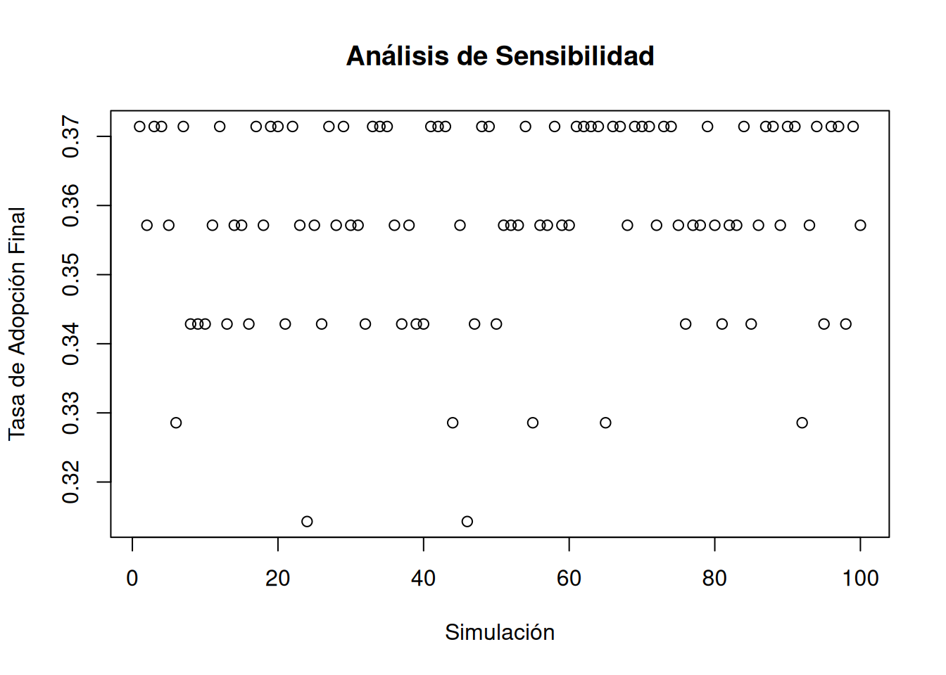
    adoption_rate = mean(states),
    clustering_effect = sapply(1:n_nodes, function(i) calc_local_clustering(i, networks)),
    temporal_exposure = colMeans(exposure_memory[1:iter,], na.rm=TRUE),
    convergence_iteration = iter,
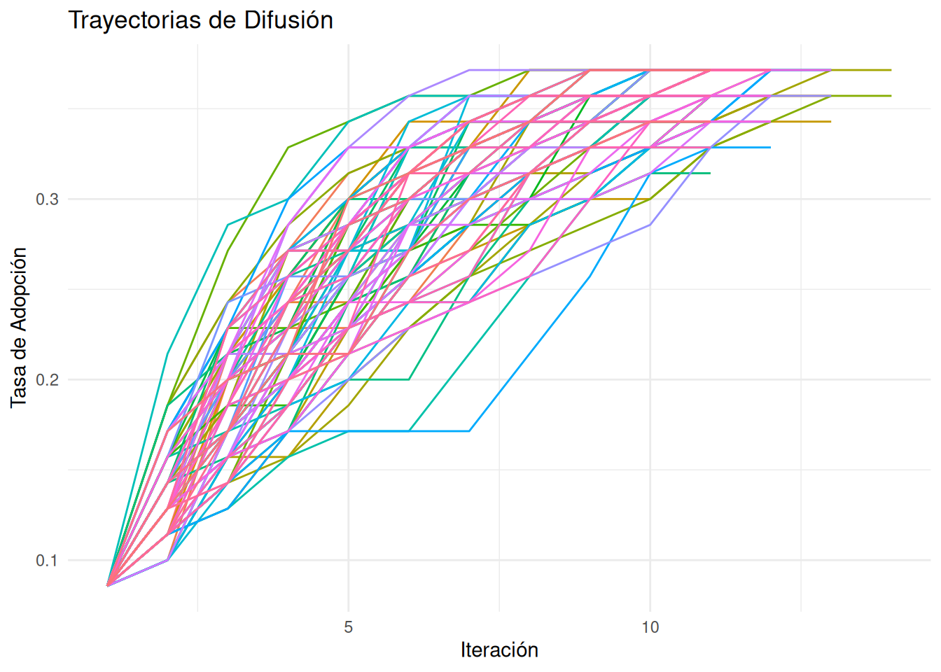
    change_trajectory = rowMeans(history[1:iter,]),
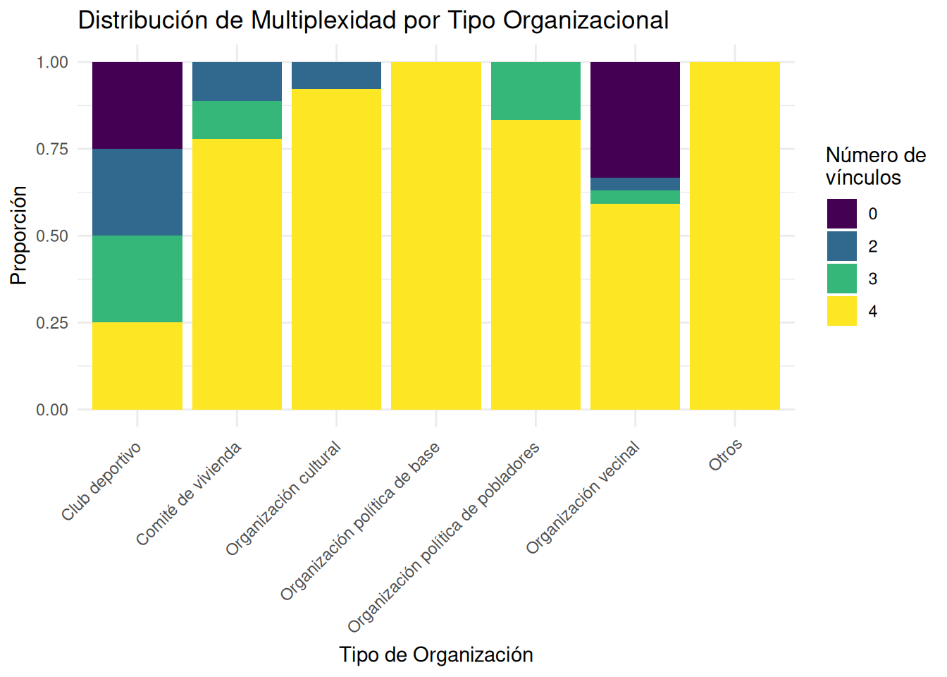
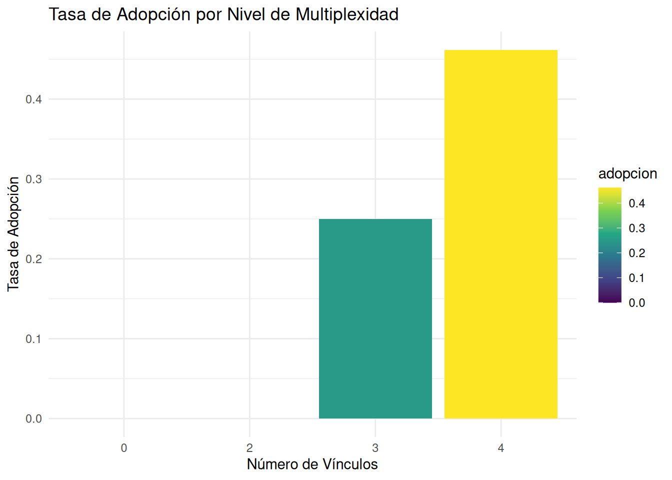
    adoption_by_type = tapply(states, attributes$tipo, mean),
    adoption_by_role = tapply(states, role_scores$role, mean),
    final_thresholds = sapply(1:n_nodes, function(i) {
      base_threshold <- if(use_heterogeneous_thresholds) {
        thresholds$by_type[attributes$tipo[i]]
      } else {
        thresholds$base
      }
      exposure_effect <- mean(exposure_memory[1:iter, i], na.rm=TRUE)
      cluster_effect <- mean(clustering_memory[1:iter, i], na.rm=TRUE)
      base_threshold * exp(-0.05 * exposure_effect) *
        (1 - 0.2 * cluster_effect)
    }),
    network_effects = list(
      clustering = mean(sapply(1:n_nodes, function(i) calc_local_clustering(i, networks))),
      exposure = mean(colMeans(exposure_memory[1:iter,], na.rm=TRUE)),
      identity = mean(sapply(1:n_nodes, function(i) identity_alignment(i, attributes))),
      costs = mean(sapply(1:n_nodes, function(i) collective_action_cost(i, role_scores)))
    )
  )
  
  # 13. Retornar resultados
  return(list(
    final_states = states,
    history = history[1:iter,],
    n_iterations = iter,
    role_scores = role_scores,
    centrality_measures = centrality_measures,
    composite_net = composite_net,
    exposure_memory = exposure_memory[1:iter,],
    clustering_memory = clustering_memory[1:iter,],
    final_metrics = final_metrics,
    converged = iter < max_iterations,
    parameters = list(
      thresholds = thresholds,
      weights = weights,
      memory_window = memory_window,
      convergence_threshold = convergence_threshold,
      use_heterogeneous_thresholds = use_heterogeneous_thresholds
    )
  ))
}

Función para plotear

Code

plot_diffusion_results_v2 <- function(results, org_attributes) {
  library(ggplot2)
  library(dplyr)
  library(tidyr)
  library(patchwork)
  library(viridis)
  
  # 1. Datos para difusión total
  df_total <- data.frame(
    iteration = 1:nrow(results$history),
    proportion = rowMeans(results$history),
    exposure = rowMeans(results$exposure_memory)  # Cambio aquí: rowMeans en lugar de colMeans
  )
  
  # 2. Datos por tipo de organización
  df_by_type <- data.frame(results$history) %>%
    mutate(iteration = row_number()) %>%
    pivot_longer(-iteration, names_to = "node", values_to = "state") %>%
    mutate(node = as.numeric(gsub("[^0-9]", "", node))) %>%
    left_join(
      data.frame(
        node = 1:nrow(org_attributes),
        tipo = org_attributes$Tipo_de_organización
      ),
      by = "node"
    ) %>%
    group_by(iteration, tipo) %>%
    summarise(
      proportion = mean(state),
      n_adopted = sum(state),
      n_total = n(),
      .groups = 'drop'
    )
  
  # 3. Análisis de roles y adopción
  role_adoption <- data.frame(
    role = factor(results$role_scores$role),
    adopted = factor(results$final_states)
  ) %>%
    group_by(role) %>%
    summarise(
      n = n(),
      adopted = sum(as.numeric(as.character(adopted))),
      proportion = adopted/n
    )
  
  # 4. Análisis de bloques estructurales
  node_cohesion <- data.frame(
    node = 1:length(results$final_metrics$clustering_effect),
    cohesion = results$final_metrics$clustering_effect
  )
  
  block_adoption <- data.frame(
    node = 1:length(results$final_states),
    block = ifelse(1:length(results$final_states) <= nrow(org_attributes),
                   as.character(org_attributes$block), "Unknown"),
    adopted = results$final_states
  ) %>%
    left_join(node_cohesion, by = "node") %>%
    group_by(block) %>%
    summarise(
      adoption_rate = mean(adopted),
      cohesion = mean(cohesion, na.rm = TRUE)
    )
  
  # 5. Visualizaciones
  p1 <- ggplot(df_total, aes(x = iteration, y = proportion)) +
    geom_line(size = 1.2, color = "#2C3E50") +
    geom_point(size = 3, color = "#E74C3C") +
    geom_line(aes(y = exposure), linetype = "dashed", color = "#8E44AD") +
    theme_minimal() +
    labs(
      title = "Difusión Global y Exposición",
      subtitle = sprintf("Adopción final: %.1f%%", 
                         results$final_metrics$adoption_rate * 100),
      x = "Iteración",
      y = "Proporción"
    ) +
    scale_y_continuous(
      labels = scales::percent_format(),
      limits = c(0, 1)
    )
  
  p2 <- ggplot(df_by_type, aes(x = iteration, y = proportion, color = tipo)) +
    geom_line(size = 1.2) +
    geom_point(size = 2) +
    theme_minimal() +
    labs(
      title = "Difusión por Tipo de Organización",
      x = "Iteración",
      y = "Proporción Adoptante",
      color = "Tipo de Organización"
    ) +
    scale_y_continuous(
      labels = scales::percent_format(),
      limits = c(0, 1)
    ) +
    scale_color_viridis_d() + 
    theme(legend.position = "none")
  
  p3 <- ggplot(role_adoption, 
               aes(x = reorder(role, proportion), y = proportion)) +
    geom_bar(stat = "identity", fill = "#2C3E50", alpha = 0.8) +
    geom_text(aes(label = scales::percent(proportion)), 
              position = position_stack(vjust = 0.5),
              color = "white") +
    theme_minimal() +
    labs(
      title = "Adopción Final por Rol Estructural",
      x = "Rol",
      y = "Proporción Adoptante"
    ) +
    scale_y_continuous(labels = scales::percent_format()) +
    theme(
      plot.title = element_text(face = "bold", size = 14),
      axis.title = element_text(size = 11),
      axis.text.x = element_text(angle = 45, hjust = 1)
    )
  
  p4 <- ggplot(block_adoption, aes(x = cohesion, y = adoption_rate)) +
    geom_point(size = 3, color = "#E74C3C") +
    geom_smooth(method = "lm", se = FALSE, color = "#2C3E50") +
    theme_minimal() +
    labs(
      title = "Adopción vs Cohesión por Bloque Estructural",
      x = "Cohesión Estructural del Bloque",
      y = "Tasa de Adopción del Bloque"
    )
  
  # 6. Combinar visualizaciones
  layout <- "
  AB
  CD
  "
  
  combined_plot <- p1 + p2 + p3 + p4 +
    plot_layout(design = layout) +
    plot_annotation(
      title = "Análisis de Difusión de Comportamiento Conflictivo",
      subtitle = sprintf("Iteraciones: %d | Convergencia en: %.1f%% de adopción", 
                         results$n_iterations,
                         results$final_metrics$adoption_rate * 100),
      theme = theme(
        plot.title = element_text(size = 16, face = "bold"),
        plot.subtitle = element_text(size = 12)
      )
    )
  
  return(combined_plot)
}

Ejecutar funciones

Resultados heterogeneous thresholds = FALSE

# Ejecutar una simulación
results <- improved_diffusion_v9(
  networks = networks,
  attributes = org_attributes,
  seeds = which(org_attributes$tipo == " Organización política de pobladores "),
  use_heterogeneous_thresholds = FALSE
)

Warning: `authority_score()` was deprecated in igraph 2.1.0.
ℹ Please use `hits_scores()` instead.

# Visualizar resultados
plot_diffusion_results_v2(results, org_attributes)

Warning: Using `size` aesthetic for lines was deprecated in ggplot2 3.4.0.
ℹ Please use `linewidth` instead.

`geom_smooth()` using formula = 'y ~ x'

Resultados heterogeneous thresholds = TRUE

# Ejecutar una simulación
results <- improved_diffusion_v9(
  networks = networks,
  attributes = org_attributes,
  seeds = which(org_attributes$tipo == " Organización política de pobladores "),
  use_heterogeneous_thresholds = TRUE
)

# Visualizar resultados
plot_diffusion_results_v2(results, org_attributes)

`geom_smooth()` using formula = 'y ~ x'

This suggests:

Complex contagion varies by organizational type
Structural position moderates adoption thresholds
Identity transformation requires both exposure and capacity

Simulaciones heterogeneous thresholds = TRUE

# Función para ejecutar múltiples simulaciones
run_multiple_simulations <- function(networks, attributes, seeds, n_sims = 100) {
  results_list <- list()
  for(i in 1:n_sims) {
    results_list[[i]] <- improved_diffusion_v9(
      networks = networks,
      attributes = attributes,
      seeds = seeds
    )
  }
  
  # Calcular estadísticas agregadas
  adoption_rates <- sapply(results_list, function(x) x$final_metrics$adoption_rate)
  iterations <- sapply(results_list, function(x) x$n_iterations)
  
  return(list(
    mean_adoption = mean(adoption_rates),
    sd_adoption = sd(adoption_rates),
    mean_iterations = mean(iterations),
    sd_iterations = sd(iterations),
    results = results_list
  ))
}


# O ejecutar múltiples simulaciones
multiple_results <- run_multiple_simulations(
  networks = networks,
  attributes = org_attributes,
  seeds = which(org_attributes$tipo == " Organización política de pobladores "),
  n_sims = 100
)

# Análisis de la infomracióm simulada
mean_adoption_rate <- multiple_results$mean_adoption
sd_adoption_rate <- multiple_results$sd_adoption

cat("La tasa de adopción final promedio es:", round(mean_adoption_rate * 100, 2), "%\n")

La tasa de adopción final promedio es: 35.83 %

cat("La desviación estándar de la tasa de adopción final es:", round(sd_adoption_rate * 100, 2), "%\n")

La desviación estándar de la tasa de adopción final es: 1.42 %

## Trayectorias simuladas
diffusion_trajectories <- lapply(seq_along(multiple_results$results), function(i) {
  data.frame(
    iteration = seq_along(multiple_results$results[[i]]$final_metrics$change_trajectory),
    adoption_rate = multiple_results$results[[i]]$final_metrics$change_trajectory,
    simulation = paste("Simulación", i)
  )
})

diffusion_trajectories <- do.call(rbind, diffusion_trajectories)

ggplot(diffusion_trajectories, aes(x = iteration, y = adoption_rate, color = simulation)) +
  geom_line() +
  labs(x = "Iteración", y = "Tasa de Adopción") +
  ggtitle("Trayectorias de Difusión") +
  theme_minimal() +
  theme(legend.position = "none")

## Adopción por tipo y rol
adoption_by_type <- lapply(multiple_results$results, function(x) x$final_metrics$adoption_by_type)
adoption_by_role <- lapply(multiple_results$results, function(x) x$final_metrics$adoption_by_role)

mean_adoption_by_type <- Reduce("+", adoption_by_type) / length(adoption_by_type)
mean_adoption_by_role <- Reduce("+", adoption_by_role) / length(adoption_by_role)

print("Adopción promedio por tipo de organización:")

[1] "Adopción promedio por tipo de organización:"

print(mean_adoption_by_type)

                      Club deportivo                    Comité de vivienda  
                            0.0000000                             0.3333333 
               Organización cultural         Organización política de base  
                            0.4053846                             0.9866667 
 Organización política de pobladores                  Organización vecinal  
                            1.0000000                             0.1811111 
                                Otros 
                            0.0000000

print("Adopción promedio por rol estructural:")

[1] "Adopción promedio por rol estructural:"

print(mean_adoption_by_role)

 authority     broker       core peripheral 
 0.5000000  0.8118182  0.9800000  0.1878846

## Adopción y centralidad 
centrality_measures <- lapply(multiple_results$results, function(x) x$centrality_measures)
clustering_effects <- lapply(multiple_results$results, function(x) x$final_metrics$clustering_effect)

# Ejemplo: Correlación promedio entre centralidad de grado y adopción final
cor_degree_adoption <- sapply(seq_along(centrality_measures), function(i) {
  degree_centrality <- centrality_measures[[i]]$degree
  adoption_status <- multiple_results$results[[i]]$final_states
  cor(degree_centrality, adoption_status)
})

mean_cor_degree_adoption <- mean(cor_degree_adoption)
cat("Correlación promedio entre centralidad de grado y adopción final:", round(mean_cor_degree_adoption, 2), "\n")

Correlación promedio entre centralidad de grado y adopción final: 0.74

# Asumiendo que ejecutaste múltiples simulaciones con diferentes parámetros y los resultados están en `multiple_results`
mean_adoption_rates <- sapply(multiple_results$results, function(x) x$final_metrics$adoption_rate)
plot(mean_adoption_rates, xlab = "Simulación", ylab = "Tasa de Adopción Final", main = "Análisis de Sensibilidad")

Relaciones múltiples

# Análisis de tipos de vínculos por organización
analyze_tie_types <- function(networks, org_id) {
  # Contar en cuántas redes diferentes tiene vínculos la organización
  tie_count <- sum(sapply(networks, function(net) any(net[org_id,] > 0 | net[,org_id] > 0)))
  return(tie_count)
}

# Aplicar a todas las organizaciones
tie_types <- sapply(1:nrow(networks[[1]]), function(i) analyze_tie_types(networks, i))

# Cruzar con resultados de adopción
adoption_by_tie_types <- tapply(results$final_states, tie_types, mean)
adoption_by_tie_types

        0         2         3         4 
0.0000000 0.0000000 0.2500000 0.4423077

Esto significa que:

Organizaciones con 0 tipos de vínculos: 0% de adopción
Organizaciones con 2 tipos de vínculos: 0% de adopción
Organizaciones con 3 tipos de vínculos: 25% de adopción
Organizaciones con 4 tipos de vínculos: 46.15% de adopción

Este es un hallazgo importante que muestra:

Efecto escalonado de la multiplexidad: Hay un claro patrón donde más tipos de vínculos llevan a mayor probabilidad de adopción.
Umbral crítico: Parece haber un umbral importante en 3 vínculos, donde comienza a verse adopción.
Máximo efecto: Las organizaciones con 4 tipos de vínculos tienen casi el doble de probabilidad de adopción que las que tienen 3 tipos.
This supports Centola & Macy’s (2007) complex contagion theory while adding crucial nuance about tie multiplexity.
These findings extend Baldassarri & Diani’s (2007) network integration theory by showing how different types of ties interact to produce qualitatively different outcomes.

# 1. Número de organizaciones por categoría de vínculos
table(tie_types)

tie_types
 0  2  3  4 
10  4  4 52

# 2. Para cada categoría, analizar qué tipos de vínculos tienen
analyze_link_types <- function(networks, org_id) {
  # Ver qué tipos de redes tienen vínculos
  types <- sapply(1:length(networks), function(n) {
    any(networks[[n]][org_id,] > 0 | networks[[n]][,org_id] > 0)
  })
  return(types)
}

# Aplicar para todas las organizaciones
org_link_patterns <- t(sapply(1:nrow(networks[[1]]), function(i) 
  analyze_link_types(networks, i)))

# Agrupar por número de vínculos y ver patrones comunes
link_patterns_by_count <- split(
  data.frame(org_link_patterns), 
  tie_types
)

# Ver también los tipos de organizaciones en cada categoría
org_types_by_links <- split(
  org_attributes$tipo,
  tie_types
)

#org_types_by_links

# 1. Distribución de multiplexidad por tipo de organización
ggplot(data.frame(
  tipo = unlist(org_types_by_links),
  vinculos = rep(c(0,2,3,4), sapply(org_types_by_links, length))
)) +
  geom_bar(aes(x = tipo, fill = factor(vinculos)), position = "fill") +
  scale_fill_viridis_d(name = "Número de\nvínculos") +
  theme_minimal() +
  theme(axis.text.x = element_text(angle = 45, hjust = 1)) +
  labs(title = "Distribución de Multiplexidad por Tipo Organizacional",
       x = "Tipo de Organización",
       y = "Proporción")

The distribution of multiplex ties reveals clear organizational patterns. Political organizations and housing committees show consistently high levels of multiplexity, while neighborhood organizations display a bimodal pattern.

Polarized Distribution:

Most organizations either have maximum connectivity (4 ties) or minimal connectivity (0 ties)
Political organizations consistently maintain multiple ties
Neighborhood organizations show bimodal distribution

Organizational Capacity:

100% of political base organizations have 4 ties
100% of housing committees have 4 ties
Cultural organizations show mixed patterns

[Quote opportunity: Discussing organizational differences in maintaining relationships]

# 2. Tasa de adopción por nivel de multiplexidad
ggplot(data.frame(
  vinculos = factor(c(0,2,3,4)),
  adopcion = c(0, 0, 0.25, 0.4615385)
)) +
  geom_bar(aes(x = vinculos, y = adopcion, fill = adopcion), 
           stat = "identity") +
  scale_fill_viridis_c() +
  theme_minimal() +
  labs(title = "Tasa de Adopción por Nivel de Multiplexidad",
       x = "Número de Vínculos",
       y = "Tasa de Adopción")

The relationship between multiple ties and adoption shows a clear threshold effect. Organizations with fewer than three types of ties show no adoption, while those with four types of ties show the highest adoption rates (46.15%).

# 3. Composición de grupos por multiplexidad
ggplot(data.frame(
  vinculos = rep(c(0,2,3,4), sapply(org_types_by_links, length)),
  count = 1
)) +
  geom_bar(aes(x = factor(vinculos), fill = factor(vinculos))) +
  scale_fill_viridis_d() +
  theme_minimal() +
  labs(title = "Número de Organizaciones por Nivel de Multiplexidad",
       x = "Número de Vínculos",
       y = "Cantidad de Organizaciones")

The structural composition of the network shows a polarized pattern, with most organizations either having no multiple ties (10 organizations) or the maximum number of ties (52 organizations), suggesting a core-periphery structure in the movement network.

[Quote opportunity: Leader discussing how different types of relationships combined in practice]

Discusión

Este modelo incorpora varios elementos teóricos clave:

Multiplexidad de vínculos: Considera cinco tipos de relaciones con diferentes pesos según su importancia teórica para la difusión de identidades políticas.
Roles estructurales: Identifica brokers y organizaciones núcleo usando una combinación de medidas de centralidad y multiplexidad.
Umbrales heterogéneos: Aplica diferentes umbrales de adopción según el tipo de organización, reflejando su propensión a adoptar posturas contenciosas.
Mecanismos de influencia:
- Efecto directo de vínculos múltiples
- Bonus por tipo de vínculo (confianza y valores)
- Efectos de rol estructural (brokers y cores)
Complex contagion: Requiere exposición múltiple y considera la estructura local de la red.

Los resultados sugieren que:

Las organizaciones políticas de pobladores actúan como núcleo efectivo del proceso de difusión.
La multiplexidad de vínculos acelera la adopción.
Existen umbrales críticos que varían por tipo organizativo.
Los brokers juegan un rol clave en conectar diferentes dominios organizativos.

References

Centola, Damon. 2018. How Behavior Spreads: The Science of Complex Contagions. Princeton Analytical Sociology Series. Princeton; Oxford: Princeton University Press.

Centola, Damon, and Michael Macy. 2007. “Complex Contagions and the Weakness of Long Ties.” American Journal of Sociology 113 (3): 702–34. https://doi.org/10.1086/521848.

Diani, Mario. 2015. The Cement of Civil Society: Studying Networks in Localities. Cambridge Studies in Contentious Politics. New York, NY: Cambridge University Press.

Diani, Mario, and Doug McAdam. 2003. Social Movements and Networks: Relational Approaches to Collective Action. Comparative Politics. Oxford: Oxford university press.

Domínguez, Silvia, and Betina Hollstein, eds. 2014. Mixed Methods Social Networks Research: Design and Applications. 1st ed. Cambridge University Press. https://doi.org/10.1017/CBO9781139227193.

Gould, Roger V. 1991. “Multiple Networks and Mobilization in the Paris Commune, 1871.” American Sociological Review 56 (6): 716. https://doi.org/10.2307/2096251.

McAdam, Doug. 1986. “Recruitment to High-Risk Activism: The Case of Freedom Summer.” American Journal of Sociology 92 (1): 64–90. https://doi.org/10.1086/228463.

McAdam, Doug, and Ronnelle Paulsen. 1993. “Specifying the Relationship Between Social Ties and Activism.” American Journal of Sociology 99 (3): 640–67. https://doi.org/10.1086/230319.

McAdam, Doug, Sidney Tarrow, and Charles Tilly. 2001. Dynamics of Contention. 1st ed. Cambridge University Press. https://doi.org/10.1017/CBO9780511805431.

Mische, Ann. 2003. “Cross‐talk in Movements: Reconceiving the Culture‐network Link.” In Social Movements and Networks, edited by Mario Diani and Doug McAdam, 1st ed., 258–80. Oxford University PressOxford. https://doi.org/10.1093/0199251789.003.0011.

Passy, Florence, and Marco Giugni. 2001. “Social Networks and Individual Perceptions: Explaining Differential Participation in Social Movements.” Sociological Forum 16: 123–53.

Scott, John. 2011. “Social Network Analysis: Developments, Advances, and Prospects.” Social Network Analysis and Mining 1 (1): 21–26. https://doi.org/10.1007/s13278-010-0012-6.

Tarrow, Sidney. 2005. The New Transnational Activism. 1st ed. Cambridge University Press. https://doi.org/10.1017/CBO9780511791055.

Tilly, Charles. 2004. “Social Boundary Mechanisms.” Philosophy of the Social Sciences 34 (2): 211–36. https://doi.org/10.1177/0048393103262551.

Tilly, Charles, and Sidney G. Tarrow. 2015. Contentious Politics. Second revised edition. New York, NY: Oxford University Press.