Descriptive Statistics and Sociodemographic Distance in ELSOC 2017-2019
R
Networks
Ego networks
Homophily
Author
Roberto Cantillan
Published
August 9, 2023
Introduction
This document provides a detailed analysis of ego-centric networks using data from ELSOC 2017 (w2) and 2019 (w4). We build a database that integrates information about egos (respondents) and their alters (named contacts), and then calculate measures of sociodemographic distance between them.
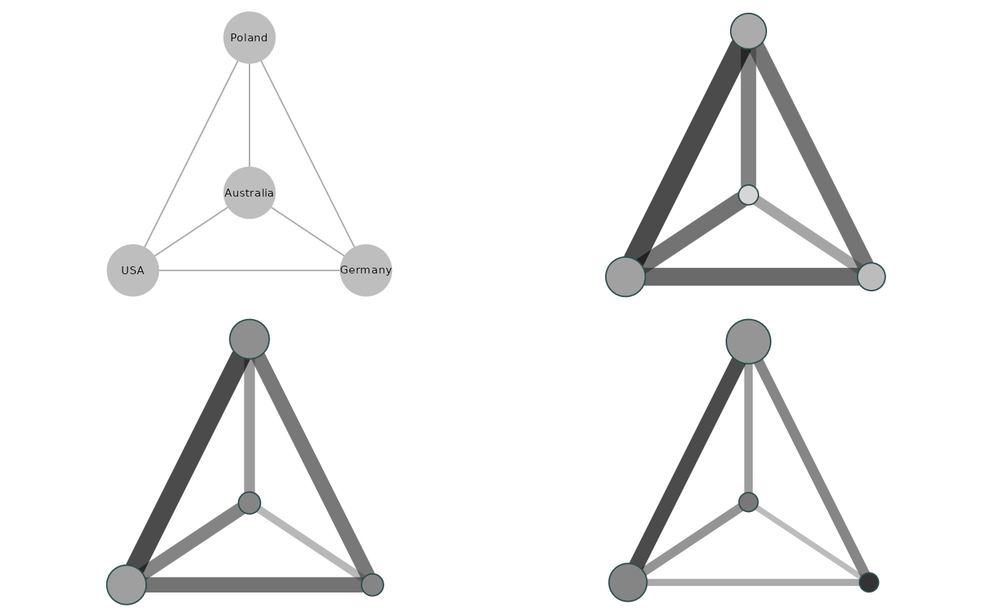
Figure 1: Egonetwork
Environment Setup
We begin by loading the required libraries. The following code uses pacman::p_load(), which installs packages if they are not already available and then loads them. Each package serves a specific purpose:
── Attaching core tidyverse packages ──────────────────────── tidyverse 2.0.0 ──
✔ dplyr     1.1.4     ✔ readr     2.1.5
✔ forcats   1.0.0     ✔ stringr   1.5.1
✔ ggplot2   3.5.2     ✔ tibble    3.3.0
✔ lubridate 1.9.4     ✔ tidyr     1.3.1
✔ purrr     1.0.2
── Conflicts ────────────────────────────────────────── tidyverse_conflicts() ──
✖ dplyr::filter() masks stats::filter()
✖ dplyr::lag()    masks stats::lag()
ℹ Use the conflicted package (<http://conflicted.r-lib.org/>) to force all conflicts to become errors
library(sjlabelled)
Attaching package: 'sjlabelled'

The following object is masked from 'package:forcats':

    as_factor

The following object is masked from 'package:dplyr':

    as_label

The following object is masked from 'package:ggplot2':

    as_label
library(sjPlot)library(texreg)
Version:  1.39.4
Date:     2024-07-23
Author:   Philip Leifeld (University of Manchester)

Consider submitting praise using the praise or praise_interactive functions.
Please cite the JSS article in your publications -- see citation("texreg").

Attaching package: 'texreg'

The following object is masked from 'package:tidyr':

    extract
library(egor)library(haven)
Attaching package: 'haven'

The following objects are masked from 'package:sjlabelled':

    as_factor, read_sas, read_spss, read_stata, write_sas, zap_labels
library(car)
Loading required package: carData

Attaching package: 'car'

The following object is masked from 'package:dplyr':

    recode

The following object is masked from 'package:purrr':

    some
library(stargazer)
Please cite as:

 Hlavac, Marek (2022). stargazer: Well-Formatted Regression and Summary Statistics Tables.
 R package version 5.2.3. https://CRAN.R-project.org/package=stargazer
library(janitor)
Attaching package: 'janitor'

The following objects are masked from 'package:stats':

    chisq.test, fisher.test
library(gridExtra)
Attaching package: 'gridExtra'

The following object is masked from 'package:dplyr':

    combine
library(ggeffects)library(kableExtra)
Attaching package: 'kableExtra'

The following object is masked from 'package:dplyr':

    group_rows
Attaching package: 'plotly'

The following object is masked from 'package:httr':

    config

The following object is masked from 'package:ggplot2':

    last_plot

The following object is masked from 'package:stats':

    filter

The following object is masked from 'package:graphics':

    layout
Data Loading
Next, we load the ELSOC datasets. These files contain information from the 2017 and 2019 waves. The .RData format preserves the original data structure, including labels and metadata:
This step is essential for network analysis. We use rename() to standardize the identifier variable across both datasets. The ‘.’ prefix in .egoID follows the conventions of the egor package for identifier variables:
a <- elsoc_2017 %>%rename(.egoID = idencuesta)
Building the Alters Database
We now turn to the most complex part: constructing the alters database. For each alter (contact mentioned by the ego), we need to extract multiple characteristics.
First Alter
The following code extracts information for the first alter mentioned by each ego. The selected variables capture:
alter_sexo: Gender of the contact (1 = male, 2 = female)
alter_edad: Age in years
alter_rel: Type of relationship with the ego (1 = family, 2 = friend, etc.)
alter_tiempo: Length of the relationship
alter_barrio: Whether the alter lives in the same neighborhood as the ego
alter_educ: Educational attainment
alter_relig: Religious affiliation
alter_ideol: Political orientation
alter_1 <- a %>% dplyr::select(.egoID, alter_sexo=r13_sexo_01, # Recodificamos nombre de variablealter_edad=r13_edad_01, # para mantener consistenciaalter_rel=r13_relacion_01, # Los sufijos _01 indicanalter_tiempo=r13_tiempo_01, # que corresponden alalter_barrio=r13_barrio_01, # primer alter mencionadoalter_educ=r13_educ_01, alter_relig=r13_relig_01, alter_ideol=r13_ideol_01)
Remaining Alters
We repeat the same process for alters 2 through 5. The only difference is the suffix in the original variable names (_02, _03, etc.). The code is repetitive but necessary to keep the data structure clear:
# Segundo alter - sufijo _02 en variables originalesalter_2 <- a %>% dplyr::select(.egoID, alter_sexo=r13_sexo_02, alter_edad=r13_edad_02, alter_rel=r13_relacion_02,alter_tiempo=r13_tiempo_02,alter_barrio=r13_barrio_02, alter_educ=r13_educ_02, alter_relig=r13_relig_02, alter_ideol=r13_ideol_02)# Tercer alter - sufijo _03alter_3 <- a %>% dplyr::select(.egoID, alter_sexo=r13_sexo_03, alter_edad=r13_edad_03, alter_rel=r13_relacion_03,alter_tiempo=r13_tiempo_03,alter_barrio=r13_barrio_03, alter_educ=r13_educ_03, alter_relig=r13_relig_03, alter_ideol=r13_ideol_03)# Cuarto alter - sufijo _04alter_4 <- a %>% dplyr::select(.egoID, alter_sexo=r13_sexo_04, alter_edad=r13_edad_04, alter_rel=r13_relacion_04,alter_tiempo=r13_tiempo_04, alter_barrio=r13_barrio_04, alter_educ=r13_educ_04, alter_relig=r13_relig_04, alter_ideol=r13_ideol_04)# Quinto alter - sufijo _05alter_5 <- a %>% dplyr::select(.egoID, alter_sexo=r13_sexo_05, alter_edad=r13_edad_05, alter_rel=r13_relacion_05,alter_tiempo=r13_tiempo_05, alter_barrio=r13_barrio_05, alter_educ=r13_educ_05, alter_relig=r13_relig_05, alter_ideol=r13_ideol_05)
Identifying Alters
To preserve the order in which alters are stored, we create a numeric variable that captures the position in which each alter was mentioned. This is crucial for later analyses that consider mention order:
# Assign sequential identifier numbersalter_1$n <-1# First alter mentionedalter_2$n <-2# Second alteralter_3$n <-3# Third alteralter_4$n <-4# Fourth alteralter_5$n <-5# Fifth alter
Building the Long-format Dataset
We then merge all alter information into a single long-format dataset. This step is crucial because it:
Enables more efficient analysis
Makes comparisons across alters easier
Is the preferred structure for many network-analysis functions
# Combine all alter datasetsalteris <-rbind(alter_1, alter_2, alter_3, alter_4, alter_5)# Order by ego ID to keep the hierarchical structurealteris <-arrange(alteris, .egoID)# Create a unique identifier for each alteralteris <-rowid_to_column(alteris, var =".altID")# Convert to tibble for easier manipulationalteris <-as_tibble(alteris)
Variable Recoding
Recoding Alter Attributes
Next, we transform the alters’ categorical variables to make the analysis easier. We use factor to convert variables into factors and Recode from the car package to relabel the values. This recoding is crucial to:
Simplify categories
Handle missing values
Create interpretable groupings
# Recode educational level# 1 = primary, 2 = secondary, 3 = vocational, 4 = universityalteris$alter_educ <-factor(Recode(alteris$alter_educ,"1=1;2:3=2;4=3;5=4;-999=NA"))# Recode religion# 1-5 represent different religious affiliationsalteris$alter_relig <-factor(Recode(alteris$alter_relig,"1=1;2=2;3=3;4=4;5=5;-999=NA"))# Recode political ideology# 1-6 represent the political spectrum from left to rightalteris$alter_ideol <-factor(Recode(alteris$alter_ideol,"1=1;2=2;3=3;4=4;5=5;6=6;-999=NA"))# Recode age into age groups# 1 = 0-18, 2 = 19-29, 3 = 30-40, 4 = 41-51, 5 = 52-62, 6 = 63+alteris$alter_edad <-factor(Recode(alteris$alter_edad,"0:18=1;19:29=2;30:40=3;41:51=4;52:62=5;63:100=6"))# Recode sex (1 = male, 2 = female)alteris$alter_sexo <-factor(Recode(alteris$alter_sexo,"1=1;2=2"))
Preparing Ego Data
We now create a dataset with information about the egos (respondents). We select variables that mirror the alter attributes so we can make direct comparisons:
# Seleccionamos y renombramos variables de egoegos <- a %>% dplyr::select(.egoID, # Respondent IDego_sexo = m0_sexo, # Respondent sexego_edad = m0_edad, # Respondent ageego_ideol = c15, # Political ideologyego_educ = m01, # Educational attainmentego_relig = m38) # Religion# Convert to tibble for easier manipulationegos <-as_tibble(egos)
Recoding Ego Variables
As with the alters, we recode ego variables to ensure comparability:
# Recode educational level# Group into four levels: primary, secondary, vocational, universityegos$ego_educ <-factor(Recode(egos$ego_educ,"1:3=1;4:5=2;6:7=3;8:10=4;-999:-888=NA"))# Recode religion# Group into five main categoriesegos$ego_relig <-factor(Recode(egos$ego_relig,"1=1;2=2;9=3;7:8=4;3:6=5;-999:-888=NA"))# Recode political ideology# Scale from 1-6 where 1 = far left and 6 = far rightegos$ego_ideol <-factor(Recode(egos$ego_ideol,"9:10=1;6:8=2;5=3;2:4=4;0:1=5;11:12=6;-999:-888=NA"))# Recode age into the same groups used for altersegos$ego_edad <-factor(Recode(egos$ego_edad,"18=1;19:29=2;30:40=3;41:51=4;52:62=5;63:100=6"))# Recode sex (1 = male, 2 = female)egos$ego_sexo <-factor(Recode(egos$ego_sexo,"1=1;2=2"))
Joining Ego and Alter Data
We combine the ego and alter datasets with a left join, which keeps all alters and their corresponding egos:
# Join the datasets using the ego ID as the keyobs <-left_join(alteris, egos, by =".egoID")# Create a case indicatorobs$case <-1# Recode missing valuesobs[obs =="-999"] <-NAobs[obs =="-888"] <-NA
Descriptive Analysis
Descriptives (alter)
We examine the frequency distribution of the alter attributes.
kbl(freq(obs$alter_educ)) %>%kable_paper()
n
%
val%
1
1362
11.0
17.8
2
3543
28.7
46.2
3
1042
8.4
13.6
4
1719
13.9
22.4
NA
4699
38.0
NA
kbl(freq(obs$alter_relig))%>%kable_paper()
n
%
val%
1
4907
39.7
60.8
2
1407
11.4
17.4
3
1128
9.1
14.0
4
251
2.0
3.1
5
373
3.0
4.6
NA
4299
34.8
NA
kbl(freq(obs$alter_ideol))%>%kable_paper()
n
%
val%
1
786
6.4
11.1
2
191
1.5
2.7
3
382
3.1
5.4
4
303
2.5
4.3
5
759
6.1
10.7
6
4644
37.6
65.7
NA
5300
42.9
NA
kbl(freq(obs$alter_edad)) %>%kable_paper()
n
%
val%
1
349
2.8
4.3
2
1477
11.9
18.3
3
1875
15.2
23.2
4
1713
13.9
21.2
5
1466
11.9
18.2
6
1186
9.6
14.7
NA
4299
34.8
NA
kbl(freq(obs$alter_sexo)) %>%kable_paper()
n
%
val%
1
3388
27.4
42
2
4678
37.8
58
NA
4299
34.8
NA
Descriptives (ego)
We review the frequency distribution of the egos’ sociodemographic attributes.
kbl(freq(obs$ego_educ)) %>%kable_paper()
n
%
val%
2985
24.1
24.1
5225
42.3
42.3
2010
16.3
16.3
2145
17.3
17.3
kbl(freq(obs$ego_relig))%>%kable_paper()
n
%
val%
1
6915
55.9
56.1
2
2495
20.2
20.2
3
1055
8.5
8.6
4
485
3.9
3.9
5
1380
11.2
11.2
NA
35
0.3
NA
kbl(freq(obs$ego_ideol))%>%kable_paper()
n
%
val%
1
915
7.4
7.5
2
1090
8.8
8.9
3
2350
19.0
19.2
4
1380
11.2
11.3
5
1075
8.7
8.8
6
5400
43.7
44.2
NA
155
1.3
NA
kbl(freq(obs$ego_edad)) %>%kable_paper()
n
%
val%
10
0.1
0.1
1865
15.1
15.1
2530
20.5
20.5
2720
22.0
22.0
2870
23.2
23.2
2370
19.2
19.2
kbl(freq(obs$ego_sexo)) %>%kable_paper()
n
%
val%
4755
38.5
38.5
7610
61.5
61.5
The tables show the frequency distribution for each sociodemographic characteristic. The columns represent: 1. The variable category 2. The absolute frequency (number of cases) 3. The percentage of the total
This information helps us understand the composition of the sample at both the ego and alter levels, and it will be essential for subsequent analyses of homophily and social distance.
Educational Homophily Analysis
We examine educational homophily with a cross-tabulation of the education levels of egos and alters. We first recode the labels to improve interpretation:
We create a heatmap to show educational homophily patterns:
# Prepare data for the heatmaptable <-as.data.frame(prop.table(table(obs$ego_educ, obs$alter_educ)))colnames(table) <-c("Ego_educ", "Alter_educ", "Prop")# Format the proportions to display percentages with two decimalstable$tooltip_text <-sprintf("Ego: %s<br>Alter: %s<br>Share: %.2f%%", table$Ego_educ, table$Alter_educ, table$Prop *100)# Create the heatmapp <-ggplot(table, aes(Ego_educ, Alter_educ)) +geom_tile(aes(fill = Prop, text = tooltip_text)) +# Add tooltip textscale_fill_gradient(low ="white", high ="black") +theme_minimal() +labs(title ="Educational Homophily Heatmap",x ="Ego Educational Level",y ="Alter Educational Level",fill ="Proportion" )# Convert to plotly and specify which variables to display in the tooltipggplotly(p, tooltip ="text")
Relationship Analysis by Type
We calculate average relationship duration by tie type:
Finally, we present a summary of the sociodemographic distances:
# Create a summary table of distanceskbl(egltable(c("sexo_dist", "edad_dist", "educ_dist", "ideol_dist", "relig_dist"),data = obs,strict =TRUE)) %>%kable_paper()
M (SD)
sexo_dist
0.36 (0.48)
edad_dist
0.65 (0.48)
educ_dist
0.65 (0.48)
ideol_dist
0.55 (0.50)
relig_dist
0.38 (0.49)
This final table shows the percentage of ego–alter dyads that differ in each sociodemographic dimension, allowing us to assess homophily patterns across characteristics.
References
Bargsted Valdés, M. A., Espinoza, V., & Plaza, A. (2020). Homophily Patterns in Chile. Papers. Revista de Sociologia, 105(4), 583. https://doi.org/10.5565/rev/papers.2617
Smith, J. A., McPherson, M., & Smith-Lovin, L. (2014). Social Distance in the United States: Sex, Race, Religion, Age, and Education Homophily among Confidants, 1985 to 2004. American Sociological Review, 79(3), 432–456. https://doi.org/10.1177/0003122414531776